Besides state estimation or localization, which provide a robot with knowledge of where it is, it’s equally important for a mobile robot to perceive its surrounding and form a knowledge of where is occupied, that’s where mapping comes in. This note covers a fundamental mapping algorithm, occupancy grid mapping.

Problem Statement

In occupancy grid mapping, a map $\mathbf{m}={\left\{m_i\right\}}_{i=1}^N$ is discretized into $N$ different cells, where each cell $m_i$ is a binary random variable that models the occupancy, and $p(m_i)$ is the probability of a cell being occupied. The map is assumed to be static. The goal is to find the belief ${\mathrm{bel}}_t(\mathbf{m})=p(\mathbf{m}\mid {\mathbf{z}}_{1:t},{\mathbf{x}}_{1:t})$, where $\mathbf{z}$ is the observation and $\mathbf{x}$ is the state of the robot.

Two assumptions are made for tractability

• The robot state ${\mathbf{x}}_t$ are known.

• The occupancy of individual cells $m_i$ are independent, and thus

At each timestep $t$, the sensor performs some measurement and provide the information of whether a cell $m_i$ is believed to be occupied or not, in terms of $p(m_i\mid {\mathbf{z}}_t,{\mathbf{x}}_t)$, which is known as the inverse sensor model.

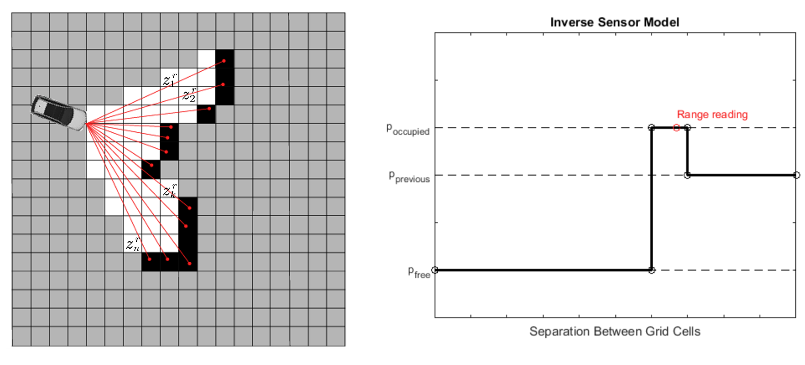
One simple inverse sensor model is shown in the figure above. Consider a laser beam range sensor that provides the reading $\mathbf{z}=(z_1^r,\dots ,z_n^r,z_1^{\varphi },\dots ,z_n^{\varphi })$, where $z_k^r$ and $z_k^{\varphi }$ are the range and bearing of the $k$-th beam. For grid $i$, let $r_i$ and ${\varphi }_i$ be the range and bearing of the grid as observed from the current robot pose $\mathbf{x}$, and $k={\mathrm{argmin}}_j\left|{\varphi }_i-z_j^{\varphi }\right|$ be the beam going through that gird. Based on the relation of a grid’s position relative to the robot, we have three different cases:

• If $r_i>\min (z_{\max },z_k^r+w_{\mathrm{grid}})$ or $\left|{\varphi }_i-z_k^{\varphi }\right|>w_{\mathrm{beam}}/2$, then return $p_{\mathrm{previous}}$, the sensor has no information about this grid.

• Else if $z_k^r<z_{\max }$ and $\left|r_i-z_k^r\right|<w_{\mathrm{grid}}$, then return $p_{\mathrm{occupied}}$, the sensor think the grid is occupied.

• Else if $z_k^r<z_{\max }$ and $r_i<z_k^r$, then return $p_{\mathrm{free}}$, the sensor think the grid is free.

where $z_{\max }$ is a sensor-specific parameter representing the maximum detectable range, $w_{\mathrm{grid}}$ is the grid size and $w_{\mathrm{beam}}$ is the width of each beam.

Mapping Algorithm

Following the Bayes filtering framework, a general algorithm can be derived for the occupancy grid mapping [2]. Starting from equation 1,

Further notice that the map $\mathbf{m}$ is independent of the robot state ${\mathbf{x}}_t$, we obtain

Similarly, for the negation

Compute the ratio of equation (2) and (3), we get

Then, change to log odds form by defining

and the product chain turns into a sum

Bayes Inference using Conjugate Prior

The previous section derived an equation for updating the belief of the map under the Bayes framework, however, it lacks the notion of uncertainty (i.e., how confident we are about the map). With the notion of conjugate prior, a proper selection of the underlying distribution function for $p(m_i)$ can both simplifies the updating rule and provide a closed form formula for uncertainty.

Recall that from Bayes rule

Bernoulli Likelihood and Beta Prior

First consider the case where the occupancy of a grid is binary, i.e., $m_i\in \{0,1\}$. Let ${\theta }_i\triangleq p(m_i=1)$ be the unknown occupancy probability. From the inverse sensor model described above, we know that each sensor measurement provide a binary result, denoted as $y_t$, where

Then, the likelihood is modeled as a Bernoulli with parameter ${\theta }_i$, i.e.,

Furthermore, if we model the prior as a Beta distribution, i.e.,

where $B(\cdot ,\cdot )$ is the beta function.

Then, it follows from the Bayes rule that the posterior is

which still follows a Beta distribution, $p({\theta }_i\mid {\mathbf{z}}_{1:t},{\mathbf{x}}_{1:t})=\mathrm{Beta}({\theta }_i;{\alpha }_t,{\beta }_t)$, where

In this case, we call beta distribution the conjugate prior for the Bernoulli likelihood.

Note that the choice of modeling the prior as a Beta distribution here is an algebraic convenience, which provides a closed-form expression for the posterior. Then the mean and covariance can be easily obtained

This note covers some of the fundamental concepts in Lie group and Lie algebra, and their applications to representing rigid body motion in robotics.

Matrix Lie Groups

A group is a set $G$ equipped with a binary map $\cdot :G\times G\to G$ satisfying the following properties:

• Closure: $\forall a,b\in G,a\cdot b\in G$.

• Associativity: $\forall a,b,c\in G,(a\cdot b)\cdot c=a\cdot (b\cdot c)$.

• Identity: $\exists e\in G,s.t.\forall a\in G,a\cdot e=e\cdot a=a$.

• Inverse: $\forall a\in G,\exists a^{-1}\in G,s.t.a\cdot a^{-1}=a^{-1}\cdot a=e$.

Here, it’s better to understand the element of a group as a kind of operation or transformation (e.g., a rotation or a rigid body transformation) rather than a number or a vector. These groups turn out to be also differentiable manifolds, which makes them Lie groups.

Special Orthogonal Group, $\mathrm{SO}(n)$

To represent a rotation formally, we need to consider the properties that define a rotation. In general, a rotation should be

• Linear, so it can be represented as a matrix $\mathbf{R}$.

• Preserves length and angles, so for any vector $\mathbf{v}$ and $\mathbf{w}$, $\mathbf{v}\cdot \mathbf{w}=(\mathbf{Rv})\cdot (\mathbf{Rw})$.

  Note, from this property,

  $${\mathbf{v}}^{\top }\mathbf{w}=(\mathbf{Rv}{)}^{\top }(\mathbf{Rw})=\mathbf{v}{\mathbf{R}}^{\top }\mathbf{Rw}$$

  which means the matrix $\mathbf{R}$ has to satisfy the following

  $$\begin{array}{c}{\mathbf{R}}^{\top }\mathbf{R}=\mathbf{I}\end{array}$$

• Preserves orientation (no mirroring), so $\det (\mathbf{R})>0$.

  Given the previous property

  $$\det ({\mathbf{R}}^{\top }\mathbf{R})=\det ({\mathbf{R}}^{\top })\cdot \det (\mathbf{R})=(\det (\mathbf{R}){)}^2=1$$

  we have

  $$\det (\mathbf{R})=1$$

In fact, these properties give rise to a group called the special orthogonal group,

which is a group of all rotations about the origin in an $n$ dimensional Euclidean space.

Special Euclidean Group, $\mathrm{SE}(n)$

The general way to represent the motion of a rigid body is a transformation that

• Preserves the Euclidean distance, $\Vert f(\mathbf{x})-f(\mathbf{y})\Vert =\Vert \mathbf{x}-\mathbf{y}\Vert$.

• Preserves the orientation.

All such transformation forms a group called the special Euclidean group, $\mathrm{SE}(n)$.

Intuitively, such transformation can be represented by a function $f:{\mathbb{R}}^n\to {\mathbb{R}}^n$, where

However, the function $f$ is not linear and thus cannot be represented by a matrix, which causes inconvenience. The general trick to solve this problem is to augment the dimension by 1. For $\mathbf{x}\in {\mathbb{R}}^n$, define $\overline{\mathbf{x}}\in {\mathbb{R}}^{n+1}$ and $\mathbf{T}\in {\mathbb{R}}^{(n+1)\times (n+1)}$ such that

so the transformation becomes matrix vector multiplication.

The special Euclidean group now can be written as

which represents all poses an object can take in an $n$ dimensional space.

Lie Algebra

A Lie algebra is a vector space $\mathfrak{g}$ together with a binary operation called the Lie bracket $[\cdot ,\cdot ]:\mathfrak{g}\times \mathfrak{g}\to \mathfrak{g}$ satisfying the following properties

• Bilinearity: $[a\mathbf{x}+b\mathbf{y},\mathbf{z}]=a[\mathbf{x},\mathbf{z}]+b[\mathbf{y},z]$, $[\mathbf{z},a\mathbf{x}+b\mathbf{y}]=a[\mathbf{z},\mathbf{x}]+b[\mathbf{z},\mathbf{y}]$.

• Alternating: $[\mathbf{x},\mathbf{x}]=0$.

• Jacobi identity: $[\mathbf{x},[\mathbf{y},\mathbf{z}]]+[\mathbf{y},[\mathbf{z},\mathbf{x}]]+[\mathbf{z},[\mathbf{x},\mathbf{y}]]=0$.

Importantly, every Lie algebra $\mathfrak{g}$ is associated to a Lie group $G$, which is the tangent space of the identity of the Lie group, denoted as $\mathfrak{g}=T_{e}G$, and it completely captures the local structure of the group. In the case of robot motion, we can think of a trajectory that lives in the Lie group while the velocity lives in the Lie algebra.

Exponential Map

Let $G$ be a Lie group and $\mathfrak{g}$ be its Lie algebra, first we need to define a few notations:

• A curve in $G$ is defined as a function $\gamma :\mathbb{R}\to G$ that maps each real number $t\in \mathbb{R}$ to an element of the group $G$.

  The derivative of $\gamma$, denoted as $\dot{\gamma }$, evaluated at a specific time $t$, $\dot{\gamma }(t)$, is a vector in the tangent space. Suppose $\gamma (t)=g$, then $\dot{\gamma }(t)\in T_{g}G$.

• Left translation: For a specific element $g\in G$, define the map $L_g:G\to G,x\mapsto gx$ as the left translation. Example: if $G=\mathrm{SO}(3)$, and $g=\mathbf{R}$, then $L_{\mathbf{R}}(\mathbf{Q})=\mathbf{RQ}$.

• Left-invariant vector field: For a vector $\xi \in \mathfrak{g}$, the left-invariant vector field $X_{\xi }$ is defined at any point $g\in G$ by $X_{\xi }(g)=(\mathrm{d}{L}_g{)}_e(\xi )$.

  Basically, start from a velocity vector $\xi \in \mathfrak{g}$, which has to stars at the origin $e$ (identity). Then, you map this velocity vector to another vector in the tangent space to a group element $g$, i.e., $T_{g}G$.

Now, suppose you have a curve ${\gamma }_{\xi }$ that starts at the identity with velocity $\xi$, then, for any $t\in \mathbb{R}$, we have

The above equation can be thought of as a “differential equation” whose solution is

Let $t=1$, the exponential map can be defined as

In robot state estimation, the Bayes filter is a probabilistic approach that estimates the state from a sequence of controls and measurements by recursively performing prediction with a motion model and correction with a measurement model. In practice, some common instantiations of the Bayes framework are the Kalman filter, information filter, and particle filter.

Mathematical Formulation of Bayes Filter

Given a sequence of measurements ${\mathrm{z}}_{1:t}={\mathbf{z}}_1,\dots ,{\mathbf{z}}_t$ and controls ${\mathbf{u}}_{1:t}={\mathbf{u}}_1,\dots ,{\mathbf{u}}_t$, and a measurement model $p({\mathbf{z}}_t\mid {\mathbf{x}}_t)$ and a motion model $p({\mathbf{x}}_t\mid {\mathbf{x}}_{t-1},{\mathbf{u}}_t)$. The Bayes filter provides a recursive framework for estimating the state ${\mathbf{x}}_t$ in terms of a probability distribution function, known as the belief $\mathrm{bel}({\mathbf{x}}_t)\triangleq p({\mathbf{x}}_t\mid {\mathbf{z}}_{1:t},{\mathbf{u}}_{1,t})$, or posterior.

The filtering algorithm is built upon two assumptions of conditional independence:

• Motion model is (1st-order) Markov:

• The measurement model is memoryless:

Given these two assumptions, we can propagate the belief over time:

We can define the predicted belief of the state at time $t$ to be the probability distribution before knowing the current measurement, i.e., $\overline{\mathrm{bel}}({\mathbf{x}}_t)\triangleq p({\mathbf{x}}_t\mid {\mathbf{z}}_{1:t-1},{\mathbf{u}}_{1:t})$. Then, the above equation becomes

where $\eta$ is the normalization coefficient, and

which is essentially a correction applied to the belief after observing the current measurement.

What remains to be done, obviously, is to predict the belief $\overline{\mathrm{bel}}({\mathbf{x}}_t)$ from the previous state:

Then, recognizing $p({\mathbf{x}}_{t-1}\mid {\mathbf{z}}_{1:t-1},{\mathbf{u}}_{1:t-1})=\mathrm{bel}({\mathbf{x}}_{t-1})$, we have

In summary, the Bayes filter provides a two-step framework for updating the belief of the current state ${\mathbf{x}}_t$ from the belief of the previous state ${\mathbf{x}}_{t-1}$:

• Prediction using the motion model (Equation 1);

• Correction using the measurement model (Equation 2).

These two steps can be performed recursively to estimate the state over time.

Kalman Filter

The Kalman filter is an instantiation of the Bayes filter with the assumption of linear Gaussian models. This means the motion model and the measurement model should be

• linear with respect to their arguments:

  Specifically, suppose $\mathbf{x}\in {\mathbb{R}}^m$ , $\mathbf{u}\in {\mathbb{R}}^n$, and $\mathbf{z}\in {\mathbb{R}}^p$. Let $\mathbf{F}\in {\mathbb{R}}^{m\times m}$, $\mathbf{G}\in {\mathbb{R}}^{m\times n}$, and $\mathbf{H}\in {\mathbb{R}}^{p\times m}$ be matrices (linear maps).

  • Motion model:

  $$\begin{array}{rlr}{\mathbf{x}}_t={\mathbf{F}}_t{\mathbf{x}}_{t-1}+{\mathbf{G}}_t{\mathbf{u}}_t+{\mathbf{w}}_t,& & {\mathbf{w}}_t\sim \mathcal{N}(0,{\mathbf{Q}}_t)\end{array}$$

  • Measurement model:

  $$\begin{array}{rlr}{\mathbf{z}}_t={\mathbf{H}}_t{\mathbf{x}}_t+{\mathbf{v}}_t,& & {\mathbf{v}}_t\sim \mathcal{N}(0,{\mathbf{R}}_t)\end{array}$$

  where $\mathbf{w}\in {\mathbb{R}}^m$ and ${\mathbf{v}}_t\in {\mathbb{R}}^p$ are white noise with variance $\mathbf{Q}\in {\mathbb{R}}^{m\times m}$ and $\mathbf{R}\in {\mathbb{R}}^{p\times p}$ , respectively.

  White noise

  A discrete-time random process (a sequence of random vectors), ${\mathbf{w}}_k$, is called white noise if

  $$\begin{array}{rlr}\mathbb{E}[{\mathbf{w}}_k{\mathbf{w}}_j^{\top }]={\mathbf{Q}}_k{\delta }_{kj},& & {\delta }_{kj}=\{\begin{array}{cc}1& k=j\\ 0& k\ne j\end{array}\end{array}$$

• following a multivariate Gaussian distribution:

  Specifically,

  • Motion model: $p({\mathbf{x}}_t\mid {\mathbf{x}}_{t-1},{\mathbf{u}}_t)=\mathcal{N}({\mathbf{x}}_t;{\mathbf{F}}_t{\mathbf{x}}_{t-1}+{\mathbf{G}}_t{\mathbf{u}}_t,{\mathbf{Q}}_t)$;
  • Measurement model: $p({\mathbf{z}}_t\mid {\mathbf{x}}_t)=\mathcal{N}({\mathbf{z}}_t;{\mathbf{H}}_t{\mathbf{x}}_t,{\mathbf{R}}_t)$.

  Note: here we need to interpret ${\mathbf{x}}_{t-1}$as a realization rather than a random variable.

  Multivariate Gaussian PDF

  $\mathcal{N}(\mathbf{x};\mathbf{\mu },\mathbf{\Sigma })$ is the probability distribution function of a random variable $\mathbf{x}\in {\mathbb{R}}^m$ that follows a Gaussian distribution with mean $\mathbf{\mu }\in {\mathbb{R}}^m$ and covariance matrix $\mathbf{\Sigma }\in {\mathbb{R}}^{m\times m}$,

  $$\mathcal{N}(\mathbf{x};\mathbf{\mu },\mathbf{\Sigma })=p(\mathbf{x})=\frac{1}{\sqrt{(2\pi {)}^m\det (\mathbf{\Sigma })}}\exp \left(-\frac{1}{2}{\left(\mathbf{x}-\mathbf{\mu }\right)}^{\top }{\mathbf{\Sigma }}^{-1}\left(\mathbf{x}-\mathbf{\mu }\right)\right)$$

Before deriving the algorithm for the Kalman filter, there are two important properties of the multivariate Gaussian distribution that are useful here.

1. Affine transformation:

   Let $\mathbf{x}$ be a random vector following a Gaussian distribution $\mathbf{x}\sim \mathcal{N}(\mathbf{\mu },\mathbf{\Sigma })$, then the random vector $\mathbf{y}=\mathbf{Ax}+\mathbf{b}$ follows a Gaussian distribution $\mathbf{y}\sim \mathcal{N}(\mathbf{A}\mathbf{\mu }+\mathbf{b},\mathbf{A\Sigma }{\mathbf{A}}^{\top })$.

   Proof

   Will come later

2. Conditional distribution:

   Let $\mathbf{y}\sim \mathcal{N}(\mathbf{\mu },\mathbf{\Sigma })$ be a random vector of dimension $m+p$. Partition $\mathbf{y}$ into a vector of dimension $m$, $\mathbf{x}\in {\mathbb{R}}^m$ and a vector of dimension $p$, $\mathbf{z}\in {\mathbb{R}}^p$, and partition $\mathbf{\mu }$ and $\mathbf{\Sigma }$ respectively,

   $$\begin{array}{c}\left[\begin{array}{c}\mathbf{x}\\ \mathbf{z}\end{array}\right]\sim \mathcal{N}\left(\left[\begin{array}{c}{\mathbf{\mu }}_x\\ {\mathbf{\mu }}_z\end{array}\right],\left[\begin{array}{cc}{\mathbf{\Sigma }}_{xx}& {\mathbf{\Sigma }}_{xz}\\ {\mathbf{\Sigma }}_{zx}& {\mathbf{\Sigma }}_{zz}\end{array}\right]\right)\end{array}$$

   then, the conditional distribution $p(\mathbf{x}\mid \mathbf{z}=z)=\mathcal{N}(\mathbf{x};{\mathbf{\mu }}_{\mathbf{x}\mid \mathbf{z}},{\mathbf{\Sigma }}_{\mathbf{x}\mid \mathbf{z}})$ , where

   $$\begin{array}{rlr}{\mathbf{\mu }}_{\mathbf{x}\mid \mathbf{z}}={\mathbf{\mu }}_x+{\mathbf{\Sigma }}_{xz}{\mathbf{\Sigma }}_{zz}^{-1}\left(z-{\mu }_z\right),& & {\mathbf{\Sigma }}_{\mathbf{x}\mid \mathbf{z}}={\mathbf{\Sigma }}_{xx}-{\mathbf{\Sigma }}_{xz}{\mathbf{\Sigma }}_{zz}^{-1}{\mathbf{\Sigma }}_{zx}\end{array}$$

   Proof

   Will come later

Now, if we assume the initial belief to be Gaussian, i.e., $\mathrm{bel}({\mathbf{x}}_0)=p({\mathbf{x}}_0)=\mathcal{N}({\mathbf{x}}_0;{\mathbf{\mu }}_0,{\mathbf{\Sigma }}_0)$. Then, from equations (1) and (2), we can see that all subsequent beliefs will be Gaussian. Thus,

Then, we only need to track ${\mathbf{\mu }}_t^{-},{\mathbf{\Sigma }}_t^{-}$ in the prediction step and ${\mathbf{\mu }}_t,{\mathbf{\Sigma }}_t$ in the correction step.

For the prediction step, use the joint distribution $p({\mathbf{x}}_t,{\mathbf{x}}_{t-1}\mid {\mathbf{u}}_{1:t},{\mathbf{z}}_{1:t-1})$ and realize

Then $\overline{\mathrm{bel}}({\mathbf{x}}_t)=p({\mathbf{x}}_t\mid {\mathbf{z}}_{1:t-1},{\mathbf{u}}_{1:t})$ can be obtained by marginalize ${\mathbf{x}}_{t-1}$,

For the correction step, form a joint distribution $p({\mathbf{x}}_t,{\mathbf{z}}_t\mid {\mathbf{u}}_{1:t},{\mathbf{z}}_{1:t-1})$ and realize

Thus, $\mathrm{bel}({\mathbf{x}}_t)=p({\mathbf{x}}_t\mid {\mathbf{z}}_t,{\mathbf{u}}_{1:t},{\mathbf{z}}_{1:t-1})$, where

Finally, normalize for numerical stability

Extended Kalman Filter (EKF)

One way to handle the case where motion model and measurement model are not linear is to approximate the functions via local linearization (Taylor expansion). Specifically, we extend the Kalman filter algorithm to cases where models are non-linear:

• Motion model

• Measurement model

Let

The EKF algorithm is

Unscented Kalman Filter (UKF)

Another non-linear Kalman filter is the unscented Kalman filter which uses deterministic sampling to approximate the distribution.

Let a function $f:{\mathbb{R}}^n\to {\mathbb{R}}^m$ be a non-linear transformation. Suppose $\mathbf{x}\in {\mathbb{R}}^n$ and $\mathbf{x}\sim \mathcal{N}(\mathbf{\mu },\mathbf{\Sigma })$. We draw a set of $n$ sigmapoints, $\mathcal{X}=\{{\mathbf{x}}_i{\}}_{i=1}^n$, and compute a weight $w_i$ for each sigma point by executing

Further let $\mathbf{y}=f(\mathbf{x})$, then $\mathbf{y}\sim \mathcal{N}({\mathbf{\mu }}^{\prime },{\mathbf{\Sigma }}^{\prime })$, where