Besides state estimation or localization, which provide a robot with knowledge of where it is, it’s equally important for a mobile robot to perceive its surrounding and form a knowledge of where is occupied, that’s where mapping comes in. This note covers a fundamental mapping algorithm, occupancy grid mapping.
Problem Statement
In occupancy grid mapping, a mapm={mi}i=1N is discretized into N different cells, where each cell mi is a binary random variable that models the occupancy, and p(mi) is the probability of a cell being occupied. The map is assumed to be static. The goal is to find the belief belt(m)=p(m∣z1:t,x1:t), where z is the observation and x is the state of the robot.
Two assumptions are made for tractability
The robot state xt are known.
The occupancy of individual cells mi are independent, and thus
At each timestep t, the sensor performs some measurement and provide the information of whether a cell mi is believed to be occupied or not, in terms of p(mi∣zt,xt), which is known as the inverse sensor model.
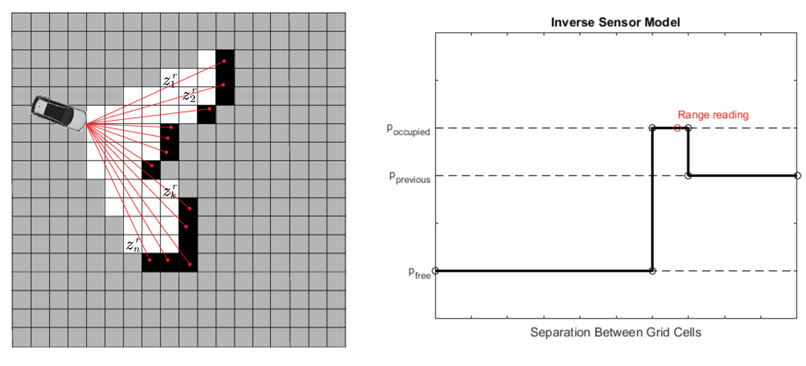
Inverse sensor model of a laser beam range sensor, image taken from [1]
One simple inverse sensor model is shown in the figure above. Consider a laser beam range sensor that provides the reading z=(z1r,…,znr,z1ϕ,…,znϕ), where zkr and zkϕ are the range and bearing of the k-th beam. For grid i, let ri and ϕi be the range and bearing of the grid as observed from the current robot pose x, and k=argminjϕi−zjϕ be the beam going through that gird. Based on the relation of a grid’s position relative to the robot, we have three different cases:
If ri>min(zmax,zkr+wgrid) or ϕi−zkϕ>wbeam/2, then return pprevious, the sensor has no information about this grid.
Else if zkr<zmax and ∣ri−zkr∣<wgrid, then return poccupied, the sensor think the grid is occupied.
Else if zkr<zmax and ri<zkr, then return pfree, the sensor think the grid is free.
where zmax is a sensor-specific parameter representing the maximum detectable range, wgrid is the grid size and wbeam is the width of each beam.
Mapping Algorithm
Following the Bayes filtering framework, a general algorithm can be derived for the occupancy grid mapping [2]. Starting from equation 1,
The previous section derived an equation for updating the belief of the map under the Bayes framework, however, it lacks the notion of uncertainty (i.e., how confident we are about the map). With the notion of conjugate prior, a proper selection of the underlying distribution function for p(mi) can both simplifies the updating rule and provide a closed form formula for uncertainty.
First consider the case where the occupancy of a grid is binary, i.e., mi∈{0,1}. Let θi≜p(mi=1) be the unknown occupancy probability. From the inverse sensor model described above, we know that each sensor measurement provide a binary result, denoted as yt, where
yt={1,0,if the inverse sensor model return poccupiedif the inverse sensor model return pfree
Then, the likelihood is modeled as a Bernoulli with parameter θi, i.e.,
which still follows a Beta distribution, p(θi∣z1:t,x1:t)=Beta(θi;αt,βt), where
αi,t=αi,t−1+ytandβi,t=βi,t−1+(1−yt)
In this case, we call beta distribution the conjugate prior for the Bernoulli likelihood.
Conjugate Distribution and Conjugate Prior [2]
If the posterior distributions are in the same probability distribution family as the prior probability distribution, the prior and posterior are then called conjugate distributions.
The prior is called a conjugate prior for the likelihood function.
Note that the choice of modeling the prior as a Beta distribution here is an algebraic convenience, which provides a closed-form expression for the posterior. Then the mean and covariance can be easily obtained
Given the simple update rule in Equation (4), the recursive Bayes framework becomes a simple counting problem: when the sensor model returns “occupied”, increment αi by 1, if the sensor model returns “free”, increment βi by 1.
Categorical Likelihood and Dirichlet Prior
Next, we can generalize the above binary occupancy mapping into a multi-categorical case using the categorical likelihood and the Dirichlet prior.
Suppose we have K different categories and each grid can be belongs to exactly one category or empty, i.e., mi∈{0,1,…,K}. Let θi=(θi,0,…,θi,K) be a vector where θi,k≜p(mi=k), and ∑k=0Kθi,k=1. Further let the measurement be a one-hot-encoded tuple yt=(yt,0,yt,1,…,yt,K) with yt,k∈{0,1} and ∑k=0Kyt,k=1, indicating which category the sensor believes cell i belongs to.
Similarly, the likelihood can be modeled as a categorical distribution
p(zt∣mi,xt)∝p(yt∣θi)=k=0∏Kθi,kyt,k
Then, we apply a Dirichlet distribution with parameterαi,t−1=(αi,t−1,0,…,αi,t−1,K)on the prior
Finally, we can write out the mapping algorithm for multi-category discrete counting sensor model
Algorithm: multi_category_discrete_CSM(mi,z,αi)Input: mi=(ri,ϕi) range and bearing of the grid from robot pose x;z=(z1r,…,znr,z1ϕ,…,znϕ,z1c,…,znc) range, bearing, and category label,where zjc∈{1,…,K} is the semantic class detected by beam j;αi=(αi,0,αi,1,…,αi,K) for cell i, where category 0 denotes free.Output: updated αi.1.b=argjminϕi−zjϕ(Find the beam going through cell mi)2.If ri>min(zmax,zbr+wgrid) or ϕi−zbϕ>wbeam/23.pass(Outside of the perception field)4.Else If zbr<zmax and ∣ri−zbr∣<wgrid5.αi,zbc←αi,zbc+1(Update: cell belongs to categoryzbc)6.Else If zbr<zmax and ri<zbr7.αi,0←αi,0+1(Update free space (category 0))
Note that if K=1, the above algorithm reduces to the binary occupancy grid mapping.
One more generalization can be made to the above discrete CSM, which is to take into account the spatial continuity. In the multi_category_discrete_CSM algorithm listed above, an observation falling into a cell grid i only updates αi of that cell and not any other cell. In reality, if a cell is observed to be occupied by a wall, then its nearby cells may also be occupied by that wall.
Let X⊂Rd be the spatial support of the map (e.g., d=2 or d=3). Define a kernel functionk(⋅,⋅):X×X→[0,1] that operates on the spatial inputs. The kernel function determines how much an observation at a location influences our belief about location x∗.
Specifically, the inverse sensor model is corrected as follows. For beam k, we construct a set of sample points S={xobs,xray(1),xray(2),…} where
xobs∈Rd is the global coordinate of the beam’s endpoint. All grids close to this endpoint is considered as occupied (or fall into some category), by a kernel-weighted factor.
xray(l)∈Rd is the global coordinate of other sample points on the beam. All grids close to any of these sample points are considered as free, by a kernel-weighted factor.
Then, during the map construction, we update the Dirichlet parameter for grid i with
αi,t,k=αi,t−1,k+x∗∈S∑k(x∗,xi)yt,k
Another benefit of continuous CSM is that we can query any point x∗ in the spatial support after the map is built, with
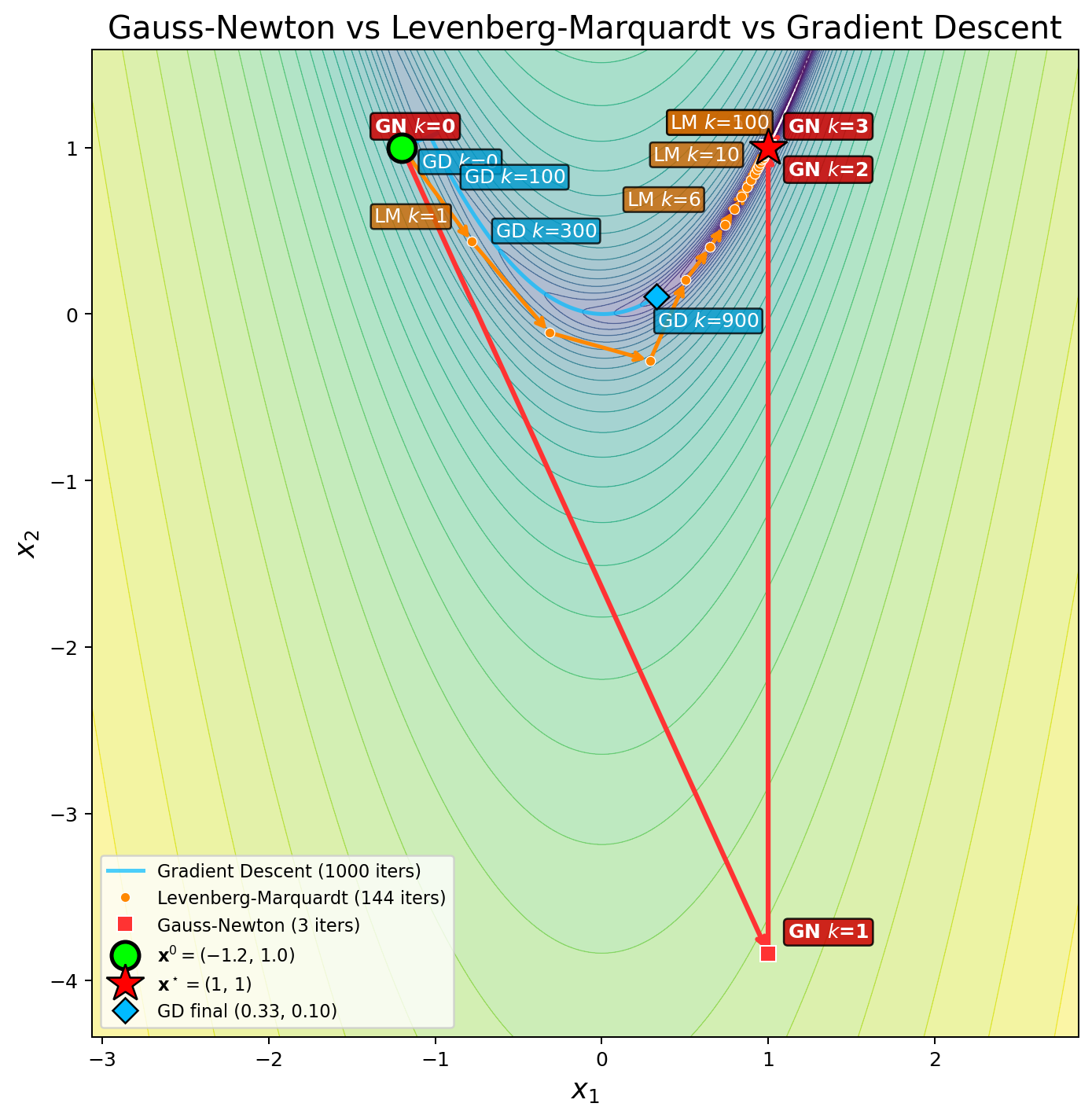
In common engineering problems, the optimization problem is to minimize the residual of a parametric model with respect to some observed data points.Given N...
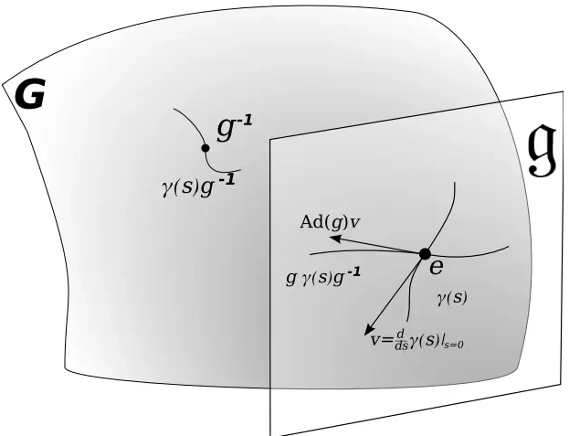
This note covers some of the fundamental concepts in Lie group and Lie algebra, and their applications to representing rigid body motion in robotics. A group...
In robot state estimation, the Bayes filter is a probabilistic approach that estimates the state from a sequence of controls and measurements by recursively ...
Two fundamental equations in acoustics areContinuity EquationThe continuity equation states that the rate at which mass enters a system is equal to the rate ...