
Lie Theory in Robot Motion
Published:
This note covers some of the fundamental concepts in Lie group and Lie algebra, and their applications to representing rigid body motion in robotics.
Matrix Lie Groups
A group is a set equipped with a binary map satisfying the following properties:
- Closure: .
- Associativity: .
- Identity: .
- Inverse: .
Here, it’s better to understand the element of a group as a kind of operation or transformation (e.g., a rotation or a rigid body transformation) rather than a number or a vector. These groups turn out to be also differentiable manifolds, which makes them Lie groups.
Special Orthogonal Group,
To represent a rotation formally, we need to consider the properties that define a rotation. In general, a rotation should be
- Linear, so it can be represented as a matrix .
- Preserves length and angles, so for any vector and , .
Note, from this property,
which means the matrix has to satisfy the following
- Preserves orientation (no mirroring), so .
Given the previous property
we have
In fact, these properties give rise to a group called the special orthogonal group,
which is a group of all rotations about the origin in an dimensional Euclidean space.
Special Euclidean Group,
The general way to represent the motion of a rigid body is a transformation that
- Preserves the Euclidean distance, .
- Preserves the orientation.
All such transformation forms a group called the special Euclidean group, .
Intuitively, such transformation can be represented by a function , where
However, the function is not linear and thus cannot be represented by a matrix, which causes inconvenience. The general trick to solve this problem is to augment the dimension by 1. For , define and such that
so the transformation becomes matrix vector multiplication.
The special Euclidean group now can be written as
which represents all poses an object can take in an dimensional space.
Lie Algebra
A Lie algebra is a vector space together with a binary operation called the Lie bracket satisfying the following properties
- Bilinearity: , .
- Alternating: .
- Jacobi identity: .
Importantly, every Lie algebra is associated to a Lie group , which is the tangent space of the identity of the Lie group, denoted as , and it completely captures the local structure of the group. In the case of robot motion, we can think of a trajectory that lives in the Lie group while the velocity lives in the Lie algebra.
Exponential Map
Let be a Lie group and be its Lie algebra, first we need to define a few notations:
- A curve in is defined as a function that maps each real number to an element of the group .
The derivative of , denoted as , evaluated at a specific time , , is a vector in the tangent space. Suppose , then .
- Left translation: For a specific element , define the map as the left translation. Example: if , and , then .
- Left-invariant vector field: For a vector , the left-invariant vector field is defined at any point by .
Basically, start from a velocity vector , which has to stars at the origin (identity). Then, you map this velocity vector to another vector in the tangent space to a group element , i.e., .
Now, suppose you have a curve that starts at the identity with velocity , then, for any , we have
The above equation can be thought of as a “differential equation” whose solution is
Let , the exponential map can be defined as
Takeaway: The exponential and logarithmic maps bridge the Lie group and its associated Lie algebra. Since Lie group is a “curved manifold” and some operations (e.g., optimizations) do not apply to it, and the Lie algebra is a flat vector space and most operations are well defined, a common paradigm is to lift group elements to Lie algebra using log map, solve the problem in Lie algebra, and bring it back to Lie group using exponential map.
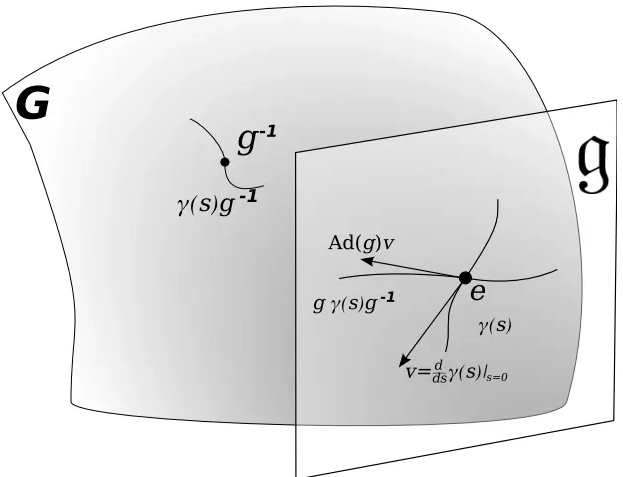
Conjugation and Adjoint Map
Let be a matrix Lie group with Lie algebra . For a specific element , the conjugation map is defined as .
The derivative of the conjugation map evaluated at the identity, is defined as the adjoint map, denoted as . For any , there exist a curve such that and , then
- A conjugation map is a change of basis transformation for an element in the Lie group.
- An adjoint map is a change of basis transformation for an element in the Lie algebra.
Angular Velocity and Twist,
Let be a smooth trajectory. By differentiating the orthogonality constraint, i.e., equation (1),
which means,
Suppose , then would be an element of the Lie algebra by definition, and we have . Therefore, the Lie algebra associated to the 3-dimensional rotation group is
which consists of all skew-symmetric matrices. Obviously, a 3 by 3 skew-symmetric matrix should look like
This means we can define a vector to represent the matrix , often denoted as or
Notice that from equation (3), and are skew-symmetric, which makes them element of . Thus, we can define two vectors such that
where is the spatial angular velocity and is the body angular velocity. From equation (4), naturally
These two equations are known as the reconstruction equation or the equation of motion. It’s better to interpret the subscript and as
- If the rotation matrix is multiplied on the left, then the velocity is in the body frame.
- If the rotation matrix is multiplied on the right, then the velocity is in the spatial frame.
Similarly, we can derive the Lie algebra of as
which is a 6-dimensional vector space, each element of which can be identified with a vector known as the twist, , often denoted as . The reconstruction equation or equation of motion can be written as
Reference
[1] T. D. Barfoot, State Estimation for Robotics. Cambridge University Press, 2024.
[2] M. Ghaffari, ROB530 Lecture Slides — Matrix Lie Groups, Robot Motion. University of Michigan, 2026.
Share on
Bluesky Facebook LinkedIn X (formerly Twitter)You May Also Enjoy
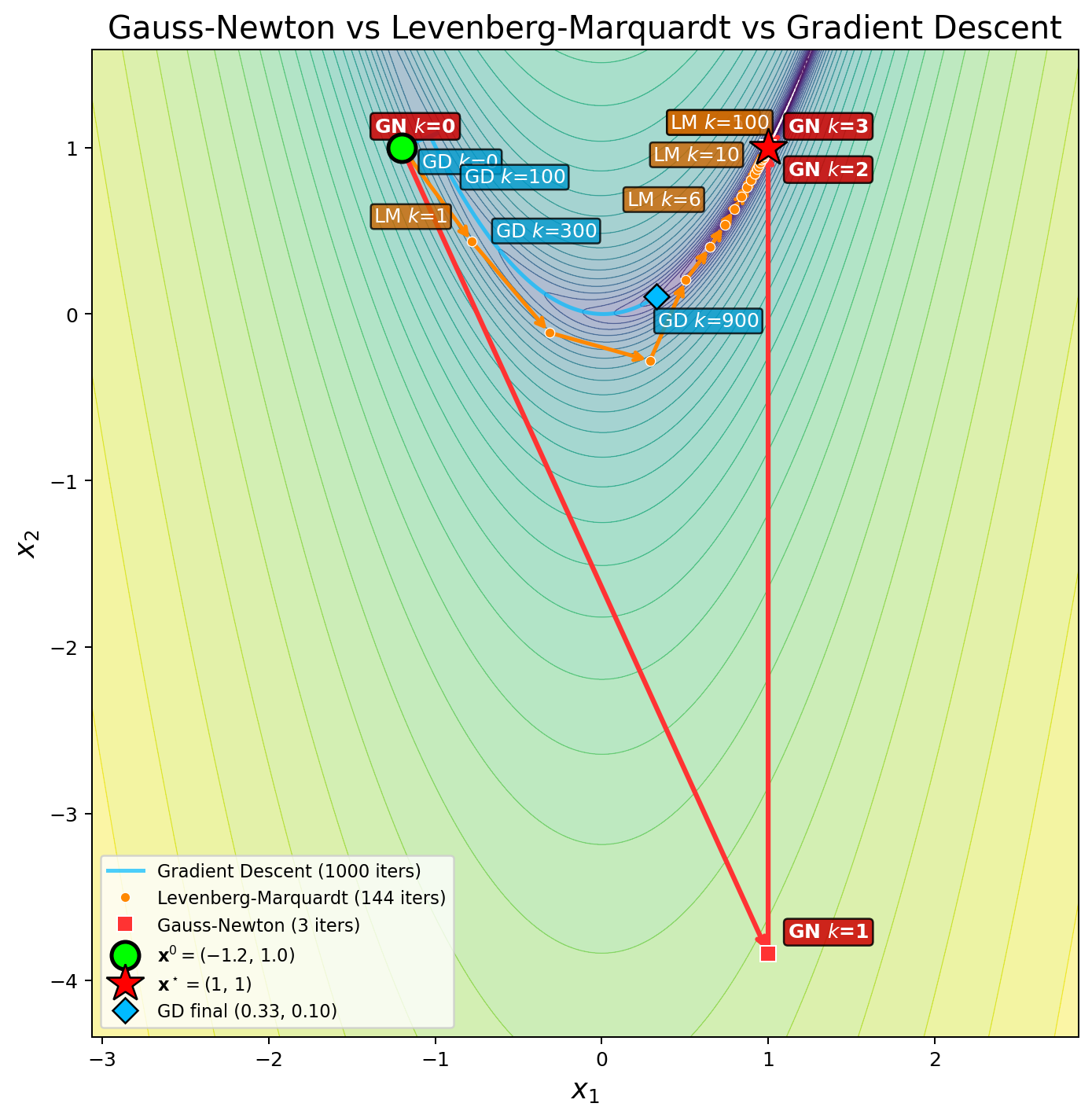
In common engineering problems, the optimization problem is to minimize the residual of a parametric model with respect to some observed data points.Given N...
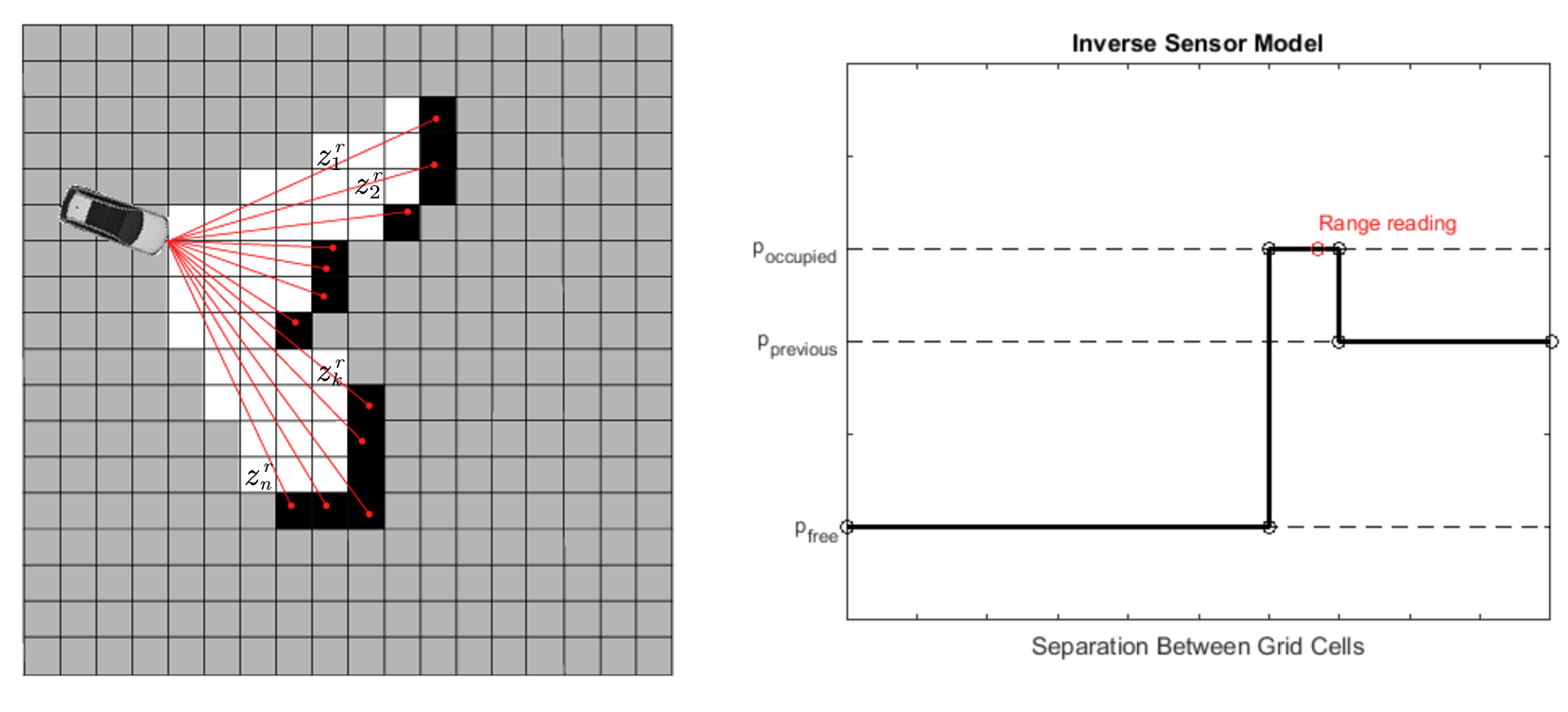
Besides state estimation or localization, which provide a robot with knowledge of where it is, it’s equally important for a mobile robot to perceive its surr...

In robot state estimation, the Bayes filter is a probabilistic approach that estimates the state from a sequence of controls and measurements by recursively ...
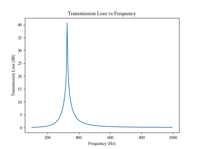
Two fundamental equations in acoustics areContinuity EquationThe continuity equation states that the rate at which mass enters a system is equal to the rate ...