Wave Theory of Sound

Two fundamental equations in acoustics are

1. Continuity Equation

The continuity equation states that the rate at which mass enters a system is equal to the rate at which mass leaves the system plus the accumulation of mass within the system.

• $\rho$ is fluid density

• $\boldsymbol{v}$ is the velocity vector of the fluid

This equation is essentially $\sum m_{in} - \sum m_{out} = \Delta m_{system}$.

2. Momentum Equation

The momentum equation states that the rate of change of momentum of a fluid element is equal to the sum of the pressure gradient force, convective acceleration, and body forces.

• $p$ is the pressure

• $\boldsymbol{g}$ is the body forces per unit mass.

This equation is essentially $F=ma$.

Wave Equation

The ambient state is characterized by its pressure $p_0$, density $\rho_0$, and fluid velocity $\boldsymbol{u}_0$. Acoustic disturbances are regarded as perturbations to the ambient state.

It can be derived from the previous two equations that the acoustic pressure $p$, which is the difference between the pressure at $(x,t)$ and the ambient pressure, satisfies the wave equation

where $c$ is the speed of propagation. For simplicity, we only consider the one-dimensional case.

Sinusoidal Plane-wave

Suppose the sound we use in this experiment is a sinusoidal wave with a constant angular frequency $\omega$. By introducing phasors, then by separation of variable, the solution is

Plug back into the wave equation to get

or simply

which is a very familiar second-order linear ODE. The general solution is

where $k=\omega/c$ is called the wave number. Finally, the total solution is

where $A,B\in\mathbb{C}$ are determined by initial and boundary conditions.

Acoustical Two-ports

Consider a model in the figure below where an acoustic element is located between two straight ducts.

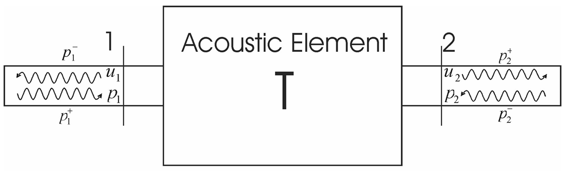
This two-port system is fully characterized by an acoustic transfer matrix, which can be written as a relation between the pressure and velocities on each side of the two-port system.

We need to consider two variables , the acoustic pressure $p$ and the volume velocity $u$ , which are analogous to voltage $V$ and current $I$ in electric circuits respectively. Then, similar to Kirchhoff’s voltage and current law, we have the continuity of pressure law and continuity of volume law.

Continuity of Pressure

This law states that acoustic pressure does not vary appreciably over distances much less than a wavelength. Consider a path from $x_1$ to $x_2$,

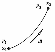
Starting from the momentum equation (Equ. 2), neglecting nonlinear term $\left(\boldsymbol{v}\cdot \nabla\right)\boldsymbol{v}$, and integrate along the path, we get,

where $\rho$ is the density of the medium, and $\boldsymbol{v}$ is the particle velocity vector.

Continuity of Volume Velocity

This law states that the net volume velocity flowing out of a volume is zero.

Starting from the continuity equation (Equ. 2), with an application of Gauss’s theorem, we obtain

Acoustic Impedance

We can define the acoustic impedance as the ratio of acoustic pressure and volume velocity,

Notice that a proper definition can be found here.

For a Helmholtz Resonator, geometry shown below,

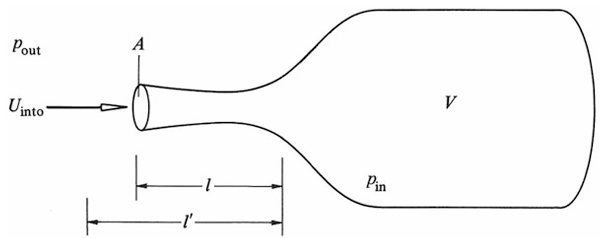
we have,

where $C_A = V/\rho c^2$ is the acoustic compliance, and $M_A = \rho l'/A$ is the acoustic inertance, $l'$ is the “effective neck length”.

Reflection and Transmission

The reason why Helmholtz Resonator can reduce noise is that it can “reflect” incident acoustic wave almost completely when the frequency of the wave is at the resonance frequency.

We define the reflection coefficient as the ratio of the intensity of the transmitted wave ($I_t$) to the incident wave ($I_i$),

It can be derived that (but I don’t know how), for Helmholtz Resonator,

At the resonance frequency,

The acoustic impedance of HR is

Then,

Thus the resonator has the potentially useful property of causing nearly total reflection of acoustic waves at frequencies near its resonance frequency. That’s why it is useful for acoustic damping.

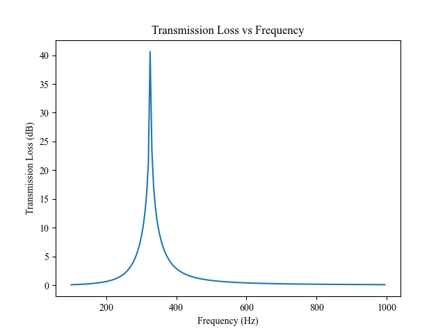
The transmission loss is defined as

By setting proper value for $A, l',\rho, c, A_D$, we can plot the transmission loss vs. frequency

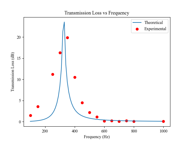
Experiment

In the experiment, we want to measure the sound transmission loss of a Helmholtz Resonator for different frequency. The setup is shown below

where test specimen is a HR connected as a side branch.

We use the loudspeaker to generate a sinusoidal wave at frequency $f$, then on the left hand side (upstream),

and on the right hand side (downstream),

Here $Ae^{i(kx+\omega t)}$ is the incident wave, $Be^{i(kx+\omega t)}$ is the reflected wave, and $Ce^{-i(kx+\omega t)}$ is the transmitted wave. By definition, the transmission loss is

To solve for $A$ and $C$, we use four microphone to measure the acoustic pressure at four different places,

Solving for $A,B,C,D$,

For convenience, we can take $s = \left|x_1-x_2\right|=\left|x_3-x_4\right|$, then the transmission loss is

The microphone record voltage signal, which is proportional to the acoustic pressure $p = p(t)$, apply Fourier transform, take $p_1(t)=Ae^{i(\omega t-kx_1)}+Be^{i(\omega t+kx_1)}$

Thus, we can see that $p_1,\dots, p_4$ are just the Fourier coefficient at the given frequency. Since we only need to ratio, by applying a Fast Fourier Transform directly to the voltage signal, and take their ratio will give the same result.