In common engineering problems, the optimization problem is to minimize the residual of a parametric model with respect to some observed data points.
Preliminaries
Given N measurements {(xi,yi)}i=1N where xi∈Rp and yi∈Rmi. We define a prediction model parametrized by θ∈Rn as h(⋅;θ):Rp→Rmi and the residual of a single datapoint as ri:Rn→Rmi, where ri(θ):=h(xi;θ)−yi. The full residual r:Rn→Rm is simply a stack of every single residuals, i.e.,
r(θ)=r1(θ)r2(θ)⋮rN(θ)∈Rm,m=i=1∑Nmi
Note that we require 𝑚≥𝑛 because otherwise the prediction model cannot be fully defined, i.e., there are infinitely many 𝜃 that perfectly fit the data.
The goal of an optimization problem is to find a model that best fits the data. To formalize this, we need to define some function f:Rn→R≥0 that properly maps the residual vector to a minimizable scalar, which is known as the objective function. In general, the function f is assumed to be continuously differentiable. Some of the common objective functions are
The following is a list of some of the theorems related to optimality conditions. Suppose f is differentiable, and define the gradient (first-order derivative) and Hessian (second-order derivative) as
Descent direction: If there is a vector d∈Rn such that ∇f(θ0)⊤d<0, then for all sufficiently small λ>0, f(θ0+λd)<f(θ0). Here, d is a descent direction of f at θ0.
Intuitively, the dot product less than 0 means that vector d is in the opposite direction as the gradient.
First-order necessary condition: If θ∗ is a local minimum, then ∇f(θ∗)=0.
Second-order necessary condition: If θ∗ is a local minimum, then ∇f(θ∗)=0 and H(θ∗)⪰0 (positive semi-definite).
Second-order sufficient condition: If ∇f(θ∗)=0 and H(θ∗)≻0 (positive definite), then θ∗ is a local minimum.
Convex function: f is convex if and only if H(θ)⪰0 for all θ.
Global minimum: Suppose f is convex, then θ⋆ is a global minimum if an only if ∇f(θ⋆)=0.
Linear Least Squares
Let A∈Rm×n be a matrix and b∈Rm be a vector, where m>n and rank(A)=n. The Linear Least Squares (LLS) optimization problem is to find the optimal solution x∈Rn to the linear system of equations Ax=b. Define the objective function as
f(x)=21∥Ax−b∥2
and the goal is to find x⋆=argminx∈Rnf(x).
First, we can write out the gradient and Hessian matrix of f, which are
Note that the last step is true because b⊤Ax∈R and b⊤Ax=(b⊤Ax)⊤=x⊤A⊤b.
Further notice that because of rank(A)=n, the Hessian matrix is positive definite (and thus invertible), i.e., A⊤A≻0. Then x⋆ is the global minimum if and only if ∇f(x⋆)=0,
A⊤Ax⋆−A⊤b=0⟹x⋆=(A⊤A)−1A⊤b
Although the above equation gives a closed-form formula for finding the global minimum x⋆, computing the inverse of A⊤A is not practical. Instead, we solve a linear system of equations
(A⊤A)x⋆=A⊤b
which is known as the normal equations.
Therefore, solving an LLS problem is basically solving a linear system of equations. Typical methods include Cholesky decomposition and QR factorization, rather than directly inverting A⊤A.
Cholesky Solver
The Cholesky decomposition of a positive-definite matrix A∈Rn×n is a decomposition into the product of an upper triangular matrix and a lower triangular matrix, i.e., A=LL⊤, where
For a linear system of equations, Ax=b, apply Cholesky decomposition and get LL⊤x=b. Then, we first let y=L⊤x, and solve Ly=b for y using forward substitution (y1→y2→⋯→yn). Specifically,
where the element of Q can be found via Gram-Schmidt diagonalization.
For a linear system of equations, Ax=b, apply QR factorization and get QRx=b. Multiply both sides by Q⊤and get Rx=Q⊤b. Let y=Q⊤b, we can solve Rx=y for x by backward substitution, i.e.,
xi=rii1(yi−j=i+1∑nrijxj),i=n−1,…,1
Non-linear Least Squares
In general, let r:Rn→Rm,m≥n be a smooth residual function. We can define an objective function f:Rn→R as
f(x)=21∥r(x)∥2=i=1∑mri2(x)
The goal is still to find the minimizer of the function f, i.e., x⋆=argminx∈Rnf(x). Unfortunately, there’s no closed-form formula for finding x⋆ as we did for the LLS problem. Common methods usually start from an initial guess, and iteratively approximate the optimum based on “descent direction” mentioned before.
Specifically, if we start with an initial guess x0, linearize around x0, and find a descending direction d. Then, we update the guess by moving along direction d , and we can expect the objective will become smaller, i.e., xk+1=xk+d and f(xk+1)<f(xk). Hopefully, this process will converge to a local minimum. Common methods include Gauss-Newton, Levenberg-Marquardt, or gradient descent, distinguished by how they compute d.
Gauss-Newton Method
The steps of the Gauss-Newton method are as follows:
Start from an initial guess x0, iterate until convergence k=0,1,2,…
Linearize the residual at the current guess xk using first-order Taylor expansion,
Solve the resulting linear least squares to find the step d⋆=argmindr(xk)+Jkd2 by solving
(Jk⊤Jk)d=−Jk⊤r(xk)
As discussed before, this is a linear system of equations, and should be solved by using Cholesky or QR decomposition rather than inverting Jk⊤Jk.
Update the current guess, xk+1=xk+d.
Implementation example:
def gauss_newton(x0, max_iter, tol):
    x = x0.copy()
    for _ in range(max_iter):
        r = residual(x)
        J = jacobian(x)
        d = np.linalg.solve(J.T @ J, -J.T @ r) # Solve (J^T J) d = -J^T r
        x = x + d
        if np.linalg.norm(d) < tol:
            break
    return x
Gradient Descent
The steps of the gradient descent method are as follows:
Start from an initial guess x0, iterate until convergence k=0,1,2,…
Compute the gradient of the objective function
∇f(xk)=Jk⊤r(xk)
Derivation
Note that
f(x)=21∥r(x)∥2=21i=1∑mri2(x)2
and the j-th entry of ∇f is
∂xj∂f=i=1∑mri(x)∂xj∂ri=Jk,j⊤r(x)
Then, stack all the entries of ∇f and we can get the result ∇f(xk)=Jk⊤r(xk).
Let the step d be the negative of the gradient, scaled by a factor called the learning rate η, i.e., d=−ηJk⊤r(xk).
Update the current guess, xk+1=xk+d.
Implementation example:
def gradient_descent(x0, max_iter, tol, eta):
    x = x0.copy()
    for _ in range(max_iter):
        r = residual(x)
        J = jacobian(x)
        d = -eta * J.T @ r # Directly set d to be along the opposite gradient
        x = x + d
        if np.linalg.norm(d) < tol:
            break
    return x
Levenberg-Marquardt Method
The step of the Levenberg-Marquardt method is as follows:
Start from an initial guess x0, iterate until convergence k=0,1,2,…
Linearize the residual at the current guess r(xk+d)=r(xk)+Jkd.
Solve a ℓ2 regularized linear least squares problem by d⋆=argmindr(xk)+Jkd2+λ∥d∥2.
def levenberg_marquardt(x0, max_iter, tol, lam):
    x = x0.copy()
    for _ in range(max_iter):
        r = residual(x)
        J = jacobian(x)
        A = J.T @ J + lam * np.eye(len(x))
        d = np.linalg.solve(A, -J.T @ r) # Solve (J^T J + λI) d = -J^T r
        x = x + d
        if np.linalg.norm(d) < tol:
            break
    return x
Note that the Levenberg-Marquardt method is an interpolation between Gauss-Newton and gradient descent.
As λ→0, it reduces to Gauss-Newton: (Jk⊤Jk+λI)→Jk⊤Jk.
As λ→∞, it reduces to gradient descent: (Jk⊤Jk+λI)→λI.
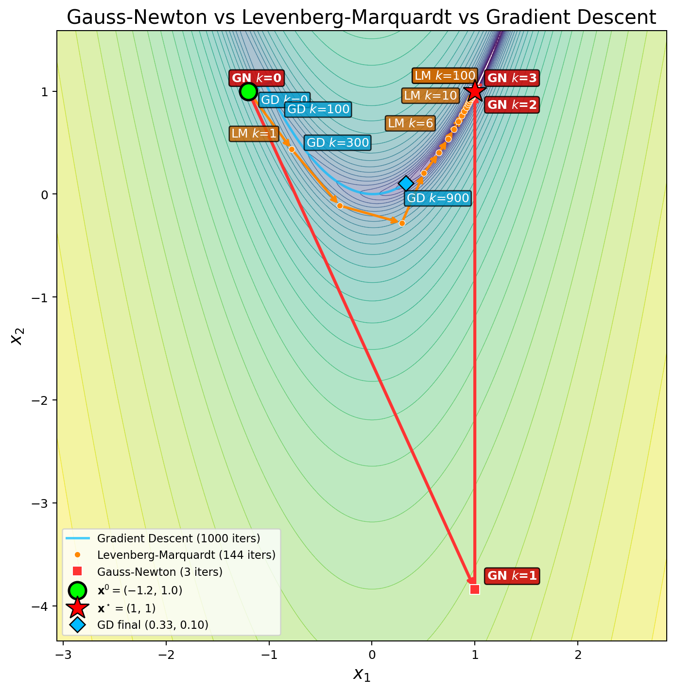
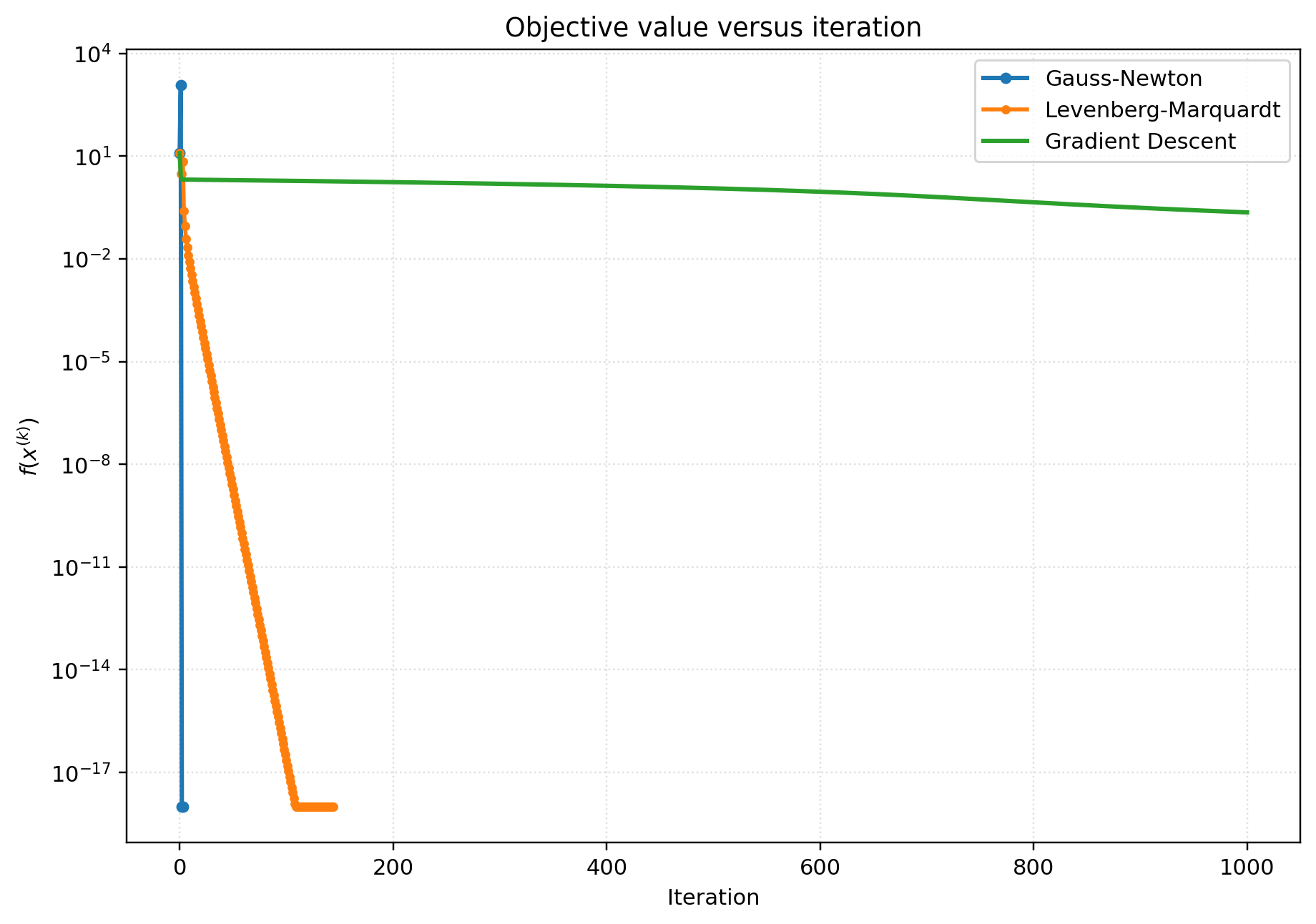
Example
Now we compare these three methods using an example. Consider the residual and objective as
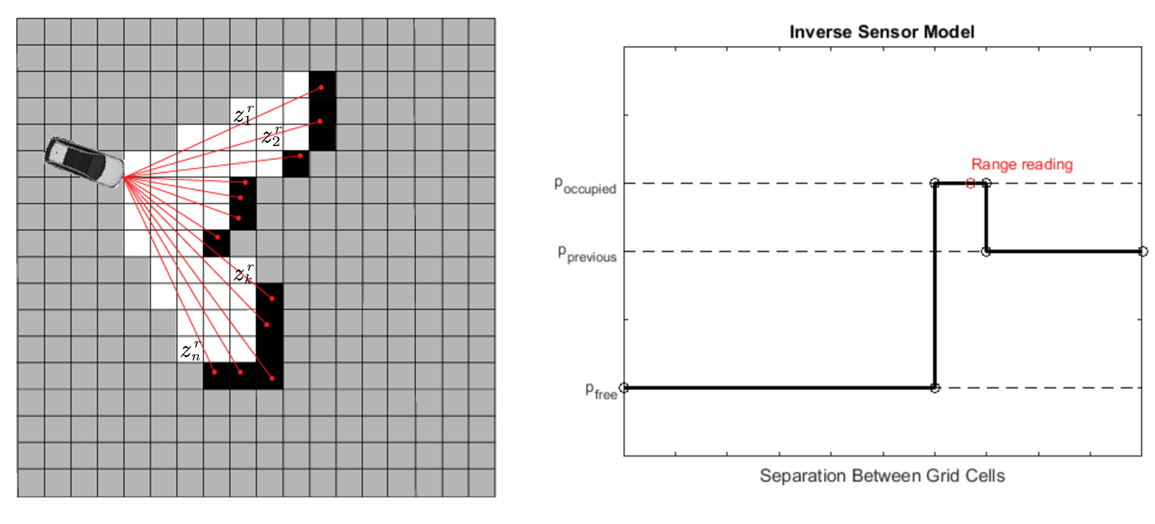
Besides state estimation or localization, which provide a robot with knowledge of where it is, it’s equally important for a mobile robot to perceive its surr...
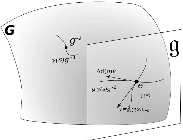
This note covers some of the fundamental concepts in Lie group and Lie algebra, and their applications to representing rigid body motion in robotics. A group...
In robot state estimation, the Bayes filter is a probabilistic approach that estimates the state from a sequence of controls and measurements by recursively ...
Two fundamental equations in acoustics areContinuity EquationThe continuity equation states that the rate at which mass enters a system is equal to the rate ...