A partial differential equation (PDE) is a relation involving one or more functions of several variables, and their partial derivatives. The order of a partial differential equation is the order of the highest partial derivative that appears in the equation.
There are three classical partial differential equations of order two which are very common in physical applications. They are known as the heat equation (1), the wave equation (2), and the Laplace equation (3).
First, it’s easy to see that the equation is linear, which means any linear combination of solutions u1(x,t),…,un(x,t) is again a solution. This suggests the following “plan” for solving this boundary-value problem.
Find as many solutions ui(x,t) as we can that satisfies the boundary conditionu(0,t)=u(l,t)=0.
Find a proper linear combination of ui to satisfies the initial conditionu(x,0)=f(x).
An important method to solve partial differential equations is separation of variables, which means we first assume u(x,t)=X(x)T(t). Then
∂t∂u=XT′,∂x2∂2u=X′′T
Plug this in the original equation and get
XT′=α2X′′T
divide both side by α2XT gives
XX′′=α2TT′
Notice that the left-hand side only depend on x, while the right-hand side only depend on t. The only way that they can equal for any x and t is that both of them are constant. Thus,
XX′′=−λ,α2TT′=−λ
By separation of variable, we have transformed a PDE into two solvable ODEs,
X′′+λX=0,T′+α2λT=0
Now, plug in the boundary condition.
0=u(0,t)=X(0)T(t),0=u(l,t)=X(l)T(t)
Since T(t)=0 (not identically zero, otherwise u would be identically zero, and we have a trivial solution), we have X(0)=X(l)=0.
Now, we only need to solve
X′′+λX=0;X(0)=0,X(l)=0
and
T′+λα2T=0
The first one is a second-order, linear, constant coefficient ODE, which we can directly write out the solution. There are three different cases:
λ=0: The general solution is X(x)=c1x+c2 for some constant c1,c2. Plug in the boundary condition, we have c1=c2=0. Thus, there are no non-trivial solution for λ=0.
λ<0: The general solution is X(x)=c1e−λx+c1e−λx for some constant c1,c2. The boundary condition implies
c1+c2=0,c1e−λl+c2e−−λl=0
This linear system of equation has non-trivial solution c1,c2 if and only if
det(1e−λl1e−−λl)=e−−λl−e−λl=0
This implies e2−λl=1, which is impossible since 2−λl>0. Therefore, there are also no non-trivial solution for λ<0.
λ>0: The general solution is X(x)=c1cosλx+c2sinλx for some constant c1,c2 The boundary condition implies
c1=0,c2sinλl=0
For c2=0, we need to have λl=nπ for positive integer n, or λn=l2n2π2. Then the equation has non-trivial solutions
X(x)=Xn(x)=sinlnπx
Then, we have the second equation,
T′+l2n2π2α2T=0
which has solution
T(t)=Tn(t)=e−α2n2π2t/l2
Hence, we have
un(x,t)=Xn(x)Tn(t)=sinlnπxe−α2n2π2t/l2
Finally, we need to use the initial condition to find a proper linear combination of un’s, i.e., find coefficients cn’s such that
u(x,t)=n=0∑∞cnsinlnπxe−α2n2π2t/l2
satisfies u(x,0)=f(x). This means that
f(x)=n=0∑∞cnsinlnπx
It’s easily seen that cn’s should be the Fourier coefficient of the pure sine expansion, which is
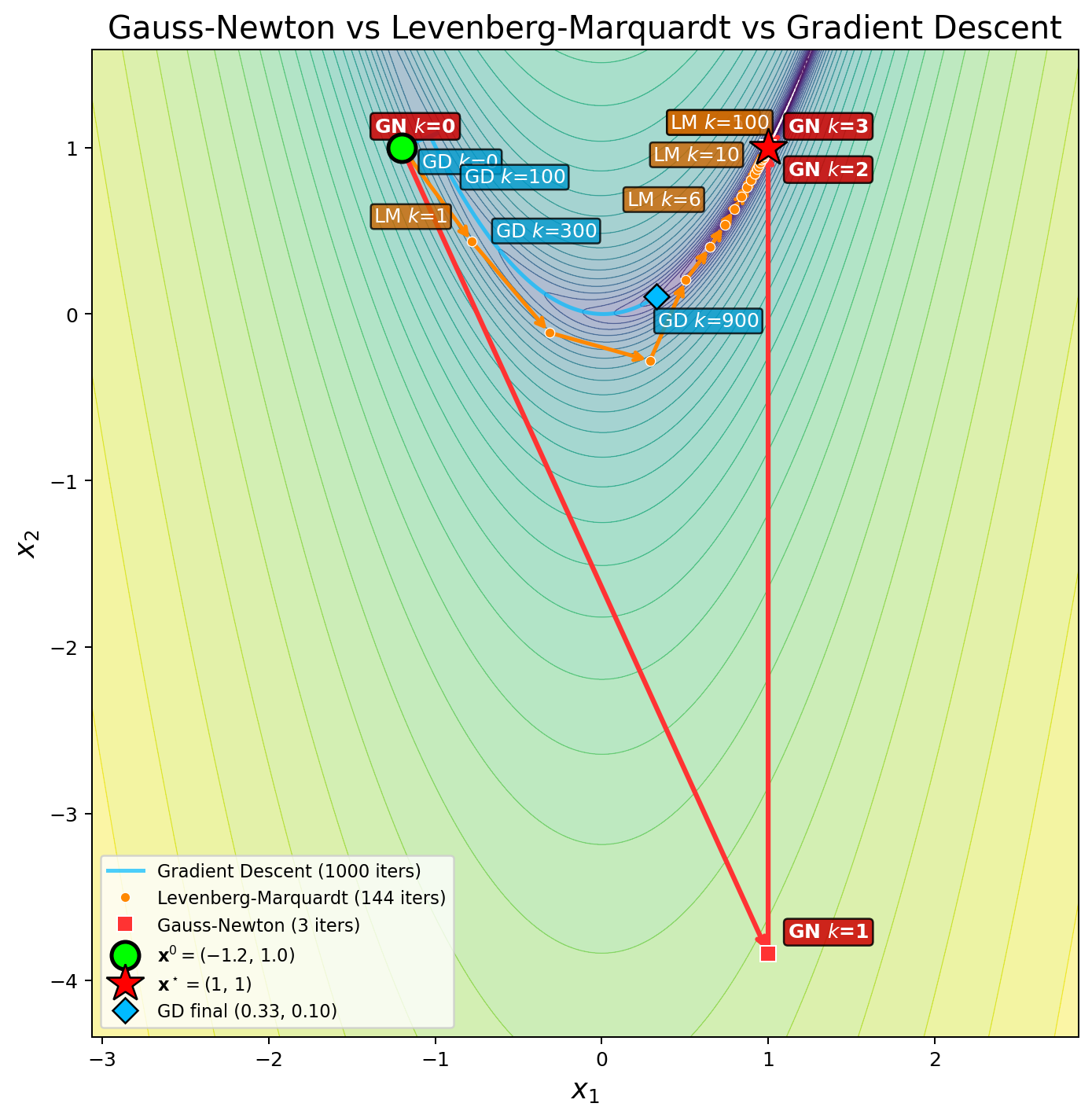
In common engineering problems, the optimization problem is to minimize the residual of a parametric model with respect to some observed data points.Given N...
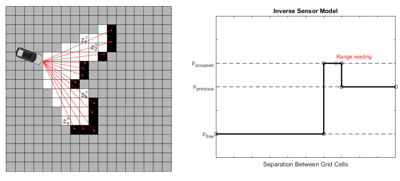
Besides state estimation or localization, which provide a robot with knowledge of where it is, it’s equally important for a mobile robot to perceive its surr...
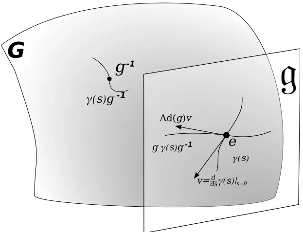
This note covers some of the fundamental concepts in Lie group and Lie algebra, and their applications to representing rigid body motion in robotics. A group...
In robot state estimation, the Bayes filter is a probabilistic approach that estimates the state from a sequence of controls and measurements by recursively ...