The Laplace transform was first introduced by Pierre-Simon Laplace in his work on probability theory. The transform turns out to have many applications in science and engineering, especially in solving linear differential equations.
The Laplace Transform
Let f(t) be defined for 0≤t<∞. The Laplace transform of f(t), which is denoted by F(s), or L{f(t)} is given by
F(s)=L{f(t)}=∫0∞e−stf(t)dt
where the improper integral is understood as
∫0∞e−stf(t)dt=A→∞lim∫0Ae−stf(t)dt
Remarks:
Two conditions that f should be satisfied to have a Laplace transform (for sufficiently large s) are
The function f(t) is of exponential order, i.e., there exist constants M and c such that for all 0≤t<∞,
∣f(t)∣≤Mect
The function f(t) is piecewise continuous, i.e., f(t) has at most a finite number of discontinuities on any interval 0≤t≤A, and both the limit from the right and the limit from the left of f exist at every point of discontinuity.
The Laplace transform doesn’t care how the function f(t) behaves when t<0, this means that different functions can have the same Laplace transform as long as they agree on t≥0.
Properties
In the following, we will assume L{f(t)}=F(s), L{g(t)}=G(s), or denotes as f(t)⇝F(s), g(t)⇝G(s). We have the following important properties.
Linearity
L{αf(t)+βg(t)}=αF(s)+βG(s)
Frequency domain derivatives
tf(t)⇝−F′(s)
tnf(t)⇝(−1)nF(n)(s)
Time domain derivatives
f′(t)⇝sF(s)−f(0)
f′′(t)⇝s2F(s)−sf(0)−f′(0)
f(n)(t)⇝snF(s)−k=1∑nsn−kf(k−1)(0)
Frequency shifting
eatf(t)⇝F(s−a)
Time shifting
u(t−a)f(t−a)⇝e−asF(s)
f(t)u(t−a)⇝e−asL(f(t+a))
where u(t) is the Heaviside step function (unit step function), and a>0.
Time scaling
f(at)⇝a1F(as)
where a>0.
Convolution
The convolution between two functions is defined as
(f∗g)(t)=∫0tf(τ)g(t−τ)dτ
Then, the Laplace transform of the convolution is the ordinary product of the Laplace transforms,
(f∗g)(t)⇝F(s)G(s)
Laplace Transform of Common Functions
The following lists the Laplace transform of some common functions:
Dirac Delta function (unit impulse)
δ(t)⇝1
δ(t−a)⇝e−as
Heaviside step function (unit step)
u(t)⇝s1
u(t−a)⇝s1e−as
Polynomial
t⇝s21
For integersn, the following two formulas hold
tn⇝sn+1n!
nt⇝sn1+11Γ(n1+1)
where
Γ(z)=∫0∞tz−1e−tdt
is the Euler’s Gamma function, with Γ(1/2)=π.
Exponential decay
e−at⇝s+a1
Sine and Cosine
sin(ωt)⇝s2+ω2ω
cos(ωt)⇝s2+ω2s
Hyperbolic Sine and Cosine
sinh(ωt)⇝s2−ω2ω
cosh(ωt)⇝s2−ω2s
Inverse Laplace Transform
The inversion of the Laplace Transform is given by the Mellin inversion formula. In particular, if f is continuous on [0,∞), continuously differentiable on (0,∞), and satisfies the condition for the Laplace transform to exist, then
is called the Bromwich integral of F, and the (positively oriented) contour is defined as
C={z∈C:Rez=β}
where β∈R is any number such that F is analytic for all z∈C with Rez≥β.
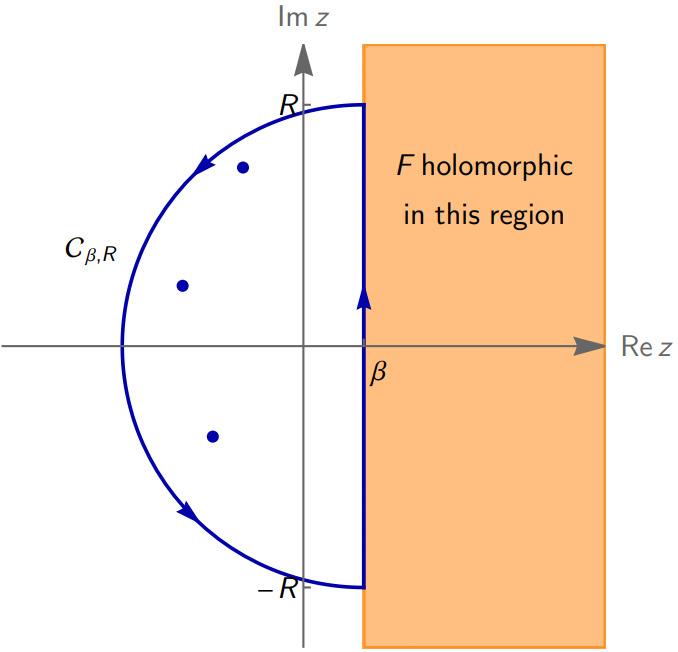
To calculate the Bromwich integral, we should consider the case when t≥0 and t<0 separately.
For t≥0, the integration contour closed on the left.
Let Γ be the straight line and Cβ,R be the semicircle (orientation indicated by the arrows). Then, by the residue theorem
∫ΓeptF(p)dp+∫Cβ,ReptF(p)dp=2πik=1∑NreszkF
Letting R→∞, the first integral be the Bromwich integral we want. For the second integral, by applying the substitution rule,
∫Cβ,ReptF(p)dp=ieβt∫CReitpF(β+ip)dp
where CR is a semi-circle of radius R in the upper half-plane. In most cases, we can use Jordan’s Lemma to show that the right-hand side goes to 0 as R→∞.
Then, the Bromwich integral of F is just the sum of all the residues of F,
2πi1∫β−i∞β+i∞eptF(p)dp=k=1∑NreszkF
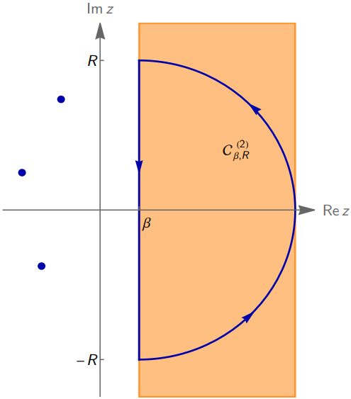
For t<0, the integration contour is closed on the left,
Let Γ be the straight line and Cβ,R(2) be the semi-circle (orientation indicated by the arrows). Using a similar argument, we see that
∫Cβ,R(2)eptF(p)dp=ieβt∫CRe−itpF(β−ip)dp
Since the integral over the whole closed contour is zero, and the orientation of the straight line is in the opposite direction, the Bromwich integral is
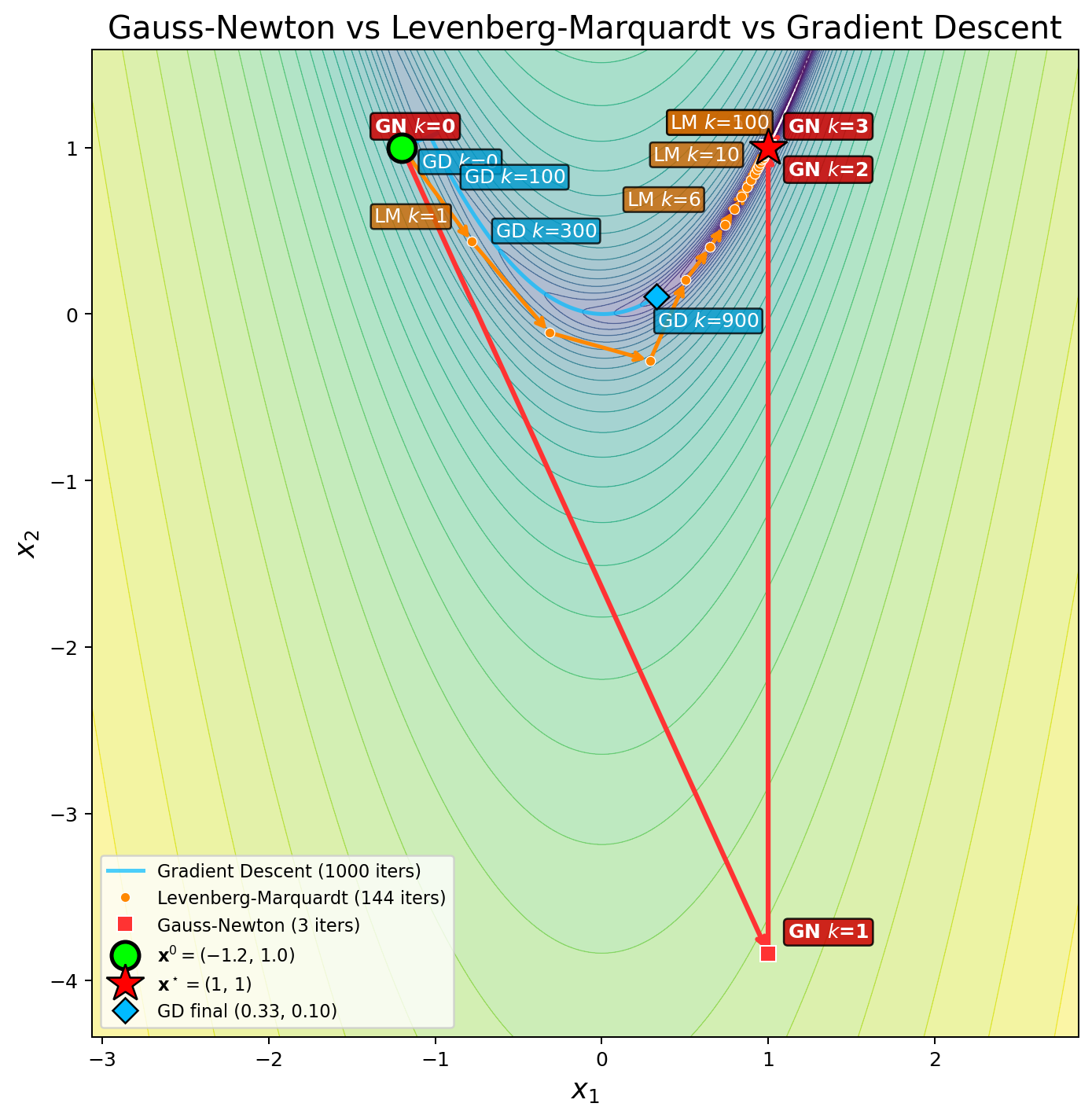
In common engineering problems, the optimization problem is to minimize the residual of a parametric model with respect to some observed data points.Given N...
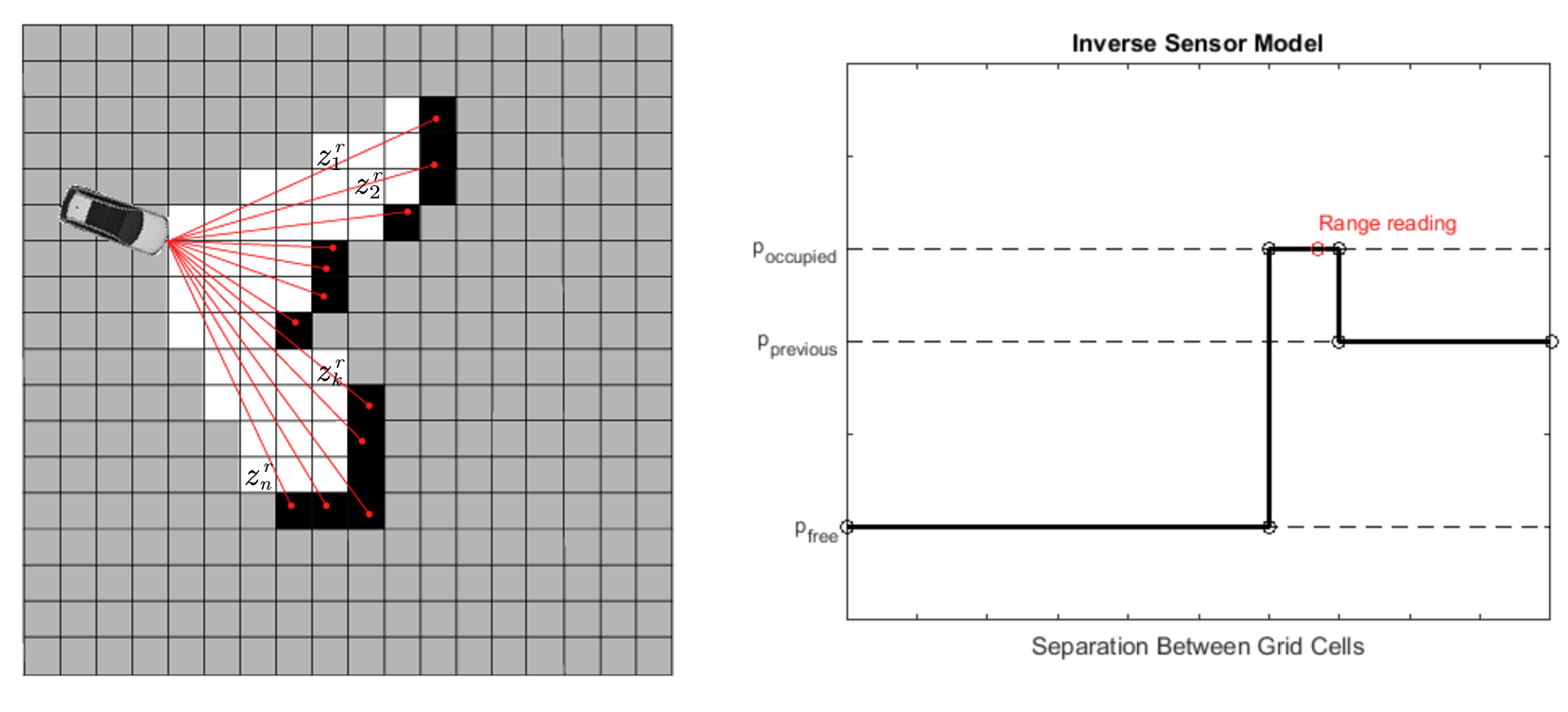
Besides state estimation or localization, which provide a robot with knowledge of where it is, it’s equally important for a mobile robot to perceive its surr...
This note covers some of the fundamental concepts in Lie group and Lie algebra, and their applications to representing rigid body motion in robotics. A group...
In robot state estimation, the Bayes filter is a probabilistic approach that estimates the state from a sequence of controls and measurements by recursively ...