An important kind of equation to learn is those linear equations, which are those can be written in the form of
Ly=b
for some linear differential operator L and unknown y. We begin by the example of second order homogeneous linear equations.
Second Order Linear Equations
Given a linear, second order, homogeneous ODE
y′′+p(t)y′+q(t)y=0
Now, we are going to show the following two things:
If y1,y2 are solution to (1), then y=c1y1+c2y2 is also a solution to (1) for some constants c1,c2∈R.
If y1 and y2 are two linearly independent solutions to (1), then all solution to (1) have the form y=c1y1+c2y2 for some constants c1,c2∈R.
The first one relies on the linearity of differential operator
L=dtd2+p(t)dtd+q(t)
We can show that this operator is linear by observing that
L(cy)=cL(y) for any constant c.
L(y1+y2)=L(y1)+L(y2).
Then, for any constant c1,c2, we have
L(c1y1+c2y2)=c1L(y1)+c2L(y2)=0
and the first one is proved.
The second one relies the Picard-Lindelof theorem also known as existence and uniqueness theorem:
Let x0∈Ω, where Ω⊂Rn is open and let t0∈I, where I⊂R be an interval.
Suppose F:Ω×I→Rn is continuous in t and Lipschitz continuous in x, i.e. there exist a constant L>0, such that for all x,y∈Ω and all t∈I,
∥F(x,t)−F(y,t)∥≤L∥x−y∥
Then, the initial value problem
x′=F(x,t)x(t0)=x0
has one and only one solution in some t interval containing t0.
An outline of the proof is as follows:
We can always construct a solution by using an iterative approximation method known as Picard iteration, which works as follows:
First, a solution to (2) will have to satisfy the integral equation
x(t)=x0+∫t0tF(x(s),s)ds
Then, by setting x(0)(t)=x0, and
x(k+1)(t)=x0+∫t0tF(x(k)(s),s)ds
yields a sequence of function x(k)(t). Then, under some condition on function F, we can use Contraction Mapping Principle to show that the sequence converges to a unique function x(t).
Algebraic Structure of Linear Equation
An interesting question to consider in the proof is that why is there exactly two independent solutions to a second linear order equation? A simple answer to this might be that since it contain second order derivative, when we solve it we shall integrate twice and each gives an integrating constant c which makes there are two constants c1,c2 to determine.
In fact, if we apply some knowledge from linear algebra, we may easy to think of the solutions as a vector space, known as solution space which happens to be 2 dimensional. And the general case would be, for a linear equation of order n, the dimension of its solution space is exactly n. Now, we want to prove this.
First notice that given an explicit ODE of order n,
x(n)(t)=f(x,x′,x′′,…,x(n−1),t)
and set new variables
x1=x,x2=x′,x3=x′′,⋯,xn=x(n−1)
Equation (3) can be written as a linear system of equations of order 1,
x1′x2′⋮xn′=x2x3⋮f(x1,x2,…,xn,t)
or, simply denoted as
x′=F(x,t)
Therefore, for any linear equation of order n, it is always equivalent to a system of n first order linear equation.
Thence, we only need to consider the first order linear system of equations,
x′=A(t)x+b(t)
where b:R→Rn, and A:R→Rn×Rn .
Consider the associated homogeneous equation
x′=A(t)x
Notice that given any two solution x1,x2, and any number λ,μ∈R, their linear combination λx1+μx2 is also a solution.
Suppose that a basis of vectors B={b1,⋯,bn}, of Rn is given and fix t0∈R. Denote by xk(t) the unique solution (theorem of Picard-Lindelof) to the initial value problem
xk′=A(t)xk,xk(t0)=bk
and denote
F={x1,⋯,xn}
Then, by superposition principle, any element of spanF is a solution to (4)
Conversely, let x be any solution to (4), and suppose that x(t0)=x0∈Rn. We have
x(t0)=x0=k=1∑nλkbk=k=1∑nλkxk(t0)
for some numbers λ1,…,λn∈R. Therefore, by theorem of Picard-Lindelof,
x=k=1∑nλkxk
This shows that the solution space is given by spanF.
Now, let’s explain why a second order linear equation will have exactly two independent solutions. For equation (1), let x1=y,x2=y′, and denote x=(x1,x2), it is equivalent to
x′=(0−p(t)1−q(t))x+(0g(t))
which is a first order linear system of equation in two dimension.
Solution to Linear System of Equations
Homogeneous, Constant Coefficients
First, consider the most basic case of linear system of equations, that is a homogeneous one with constant coefficients:
x′=Ax,x(0)=x0
where x:R→Rn and A∈M(n×n;R).
With proper definition, it can be shown that the solution to the initial value problem (6) is
x(t)=eAtx0
where
eAt=I+k=1∑∞k!Aktk
Now, the problem is how to calculate this matrix exponential. Recall from linear algebra that diagonal matrix, or Jordan matrix, are relative easy to calculate the matrix exponential. Fortunately, we have the Jordan Normal Form theorem which states that every complex matrix is similar to a Jordan matrix, i.e., for any matrix A, there exists a matrix U and a Jordan matrix J such that
be a Jordan matrix, where Jki(λi) is a Jordan block of size ki and diagonal element λi, i.e.,
Jki(λi)=λi01⋱01λi
It’s easy to show that
eJt=eJk1(λ1)0⋱0eJkm(λm)
Hence, it’s sufficient to calculate the exponential of Jordan blocks. Notice that
Jk(λ)=λI+N
where N is some nilpotent matrix whose power will vanish after finite many times, and that unit matrix commutes with any other matrix in terms of multiplication, i.e., IN=NI. Therefore,
However, the above calculation seems too complicated that it would be impractical. If we trace back what we are actually doing, we know that we are actually finding a basis of the solution space.
From previous discussion of the structure of the solution, we know immediately that for any basis B={b1,⋯,bn} of Rn, the system of functions F={eAtb1,⋯,eAtbn} is a fundamental system of solution. We collect them into one matrix and denoted as X, and is also called the fundamental matrix.
It turns out that if we choose the basis wisely, we don’t even need to calculate the whole eAt to get a fundamental matrix. From theory of Jordan normal form, we know that there exists a basis consists of (generalized) eigenvectorsU={u1,⋯,un}, such that the Jordan matrix of A is given by J=U−1AU. Using this basis, we have the fundamental matrix simply given by
X(t)=UeJt
The columns of X will therefore be the fundamental system of solutions.
Inhomogeneous, Constant Coefficients
Next, we solve an inhomogeneous equation with constant coefficients. The general solution is the superposition of a particular solution and the solution to the associated homogeneous equation.
Consider the following linear system of differential equation
x′=Ax+b(t)
suppose F={x1,⋯,xn} is a fundamental system for the associated homogeneous equation, then the general solution is given by
x(t;c1,⋯,cn)=k=1∑nckxk(t)+eAt∫e−Atb(t)dt
Variable Coefficients
There is no general method of solving homogeneous equations with variable coefficients,
x′=A(t)x
However, if we are given a fundamental system of solution F={x1,⋯,xn}, then we can find a particular solution to the inhomogeneous equation
Let X(t)=(x1(t),⋯,xn(t)) be the fundamental matrix, and c(t)=c1(t)c2(t)⋮cn(t) then the previous equation is indeed the following linear system of equation
Xc′=b
Using Cramer’s rule, we can find the solution to ck′(t).
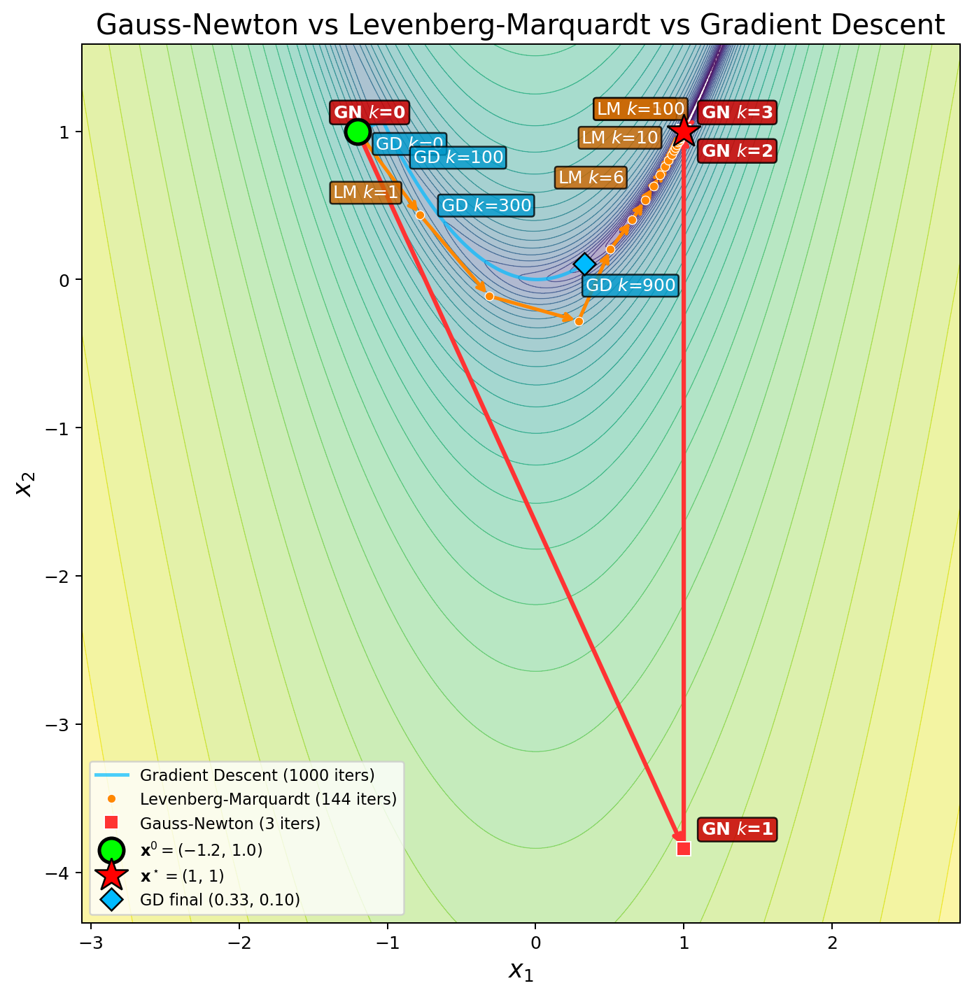
In common engineering problems, the optimization problem is to minimize the residual of a parametric model with respect to some observed data points.Given N...
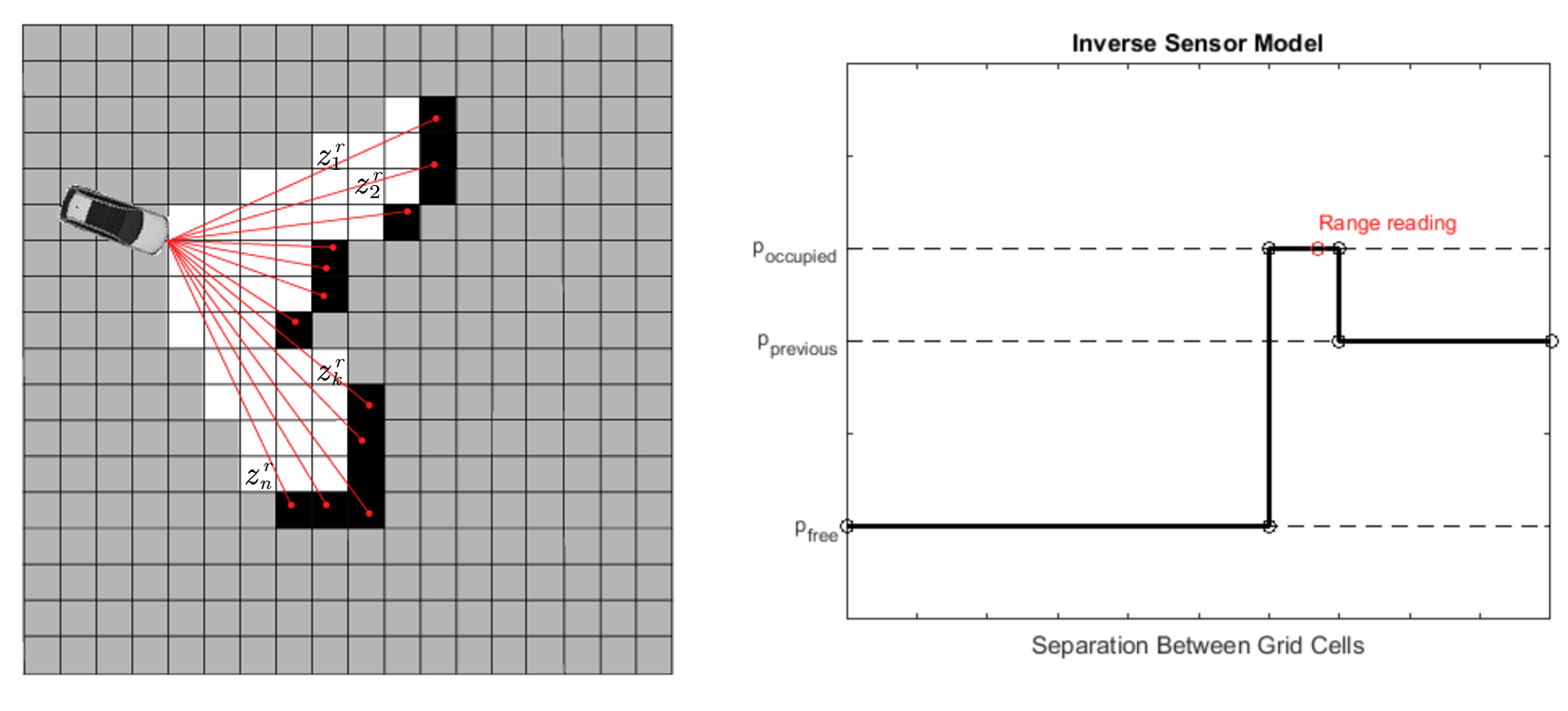
Besides state estimation or localization, which provide a robot with knowledge of where it is, it’s equally important for a mobile robot to perceive its surr...
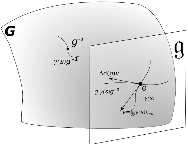
This note covers some of the fundamental concepts in Lie group and Lie algebra, and their applications to representing rigid body motion in robotics. A group...
In robot state estimation, the Bayes filter is a probabilistic approach that estimates the state from a sequence of controls and measurements by recursively ...