
Solving First and Second Order ODEs
Published:
First Order ODEs
First order ODE is equations that has the highest derivative of order one. It takes the form
The general solution to this equation is some function that satisfies the equation.
Separable Equation
A separable equation is of the form
Linear Equation
A linear equation is of the form
For now, we assume for all , then the equation above is simplified into
- If for all , it is called a homogeneous equation;
- Otherwise, it is called an inhomogeneous equation.
Homogeneous
A homogeneous linear equation is of the form
which is a separable equation. The general solution to it is
If given an initial condition , then the solution is
Inhomogeneous
An inhomogeneous linear equation is of the form
Let
and multiply , which is called the integrating factor, to both sides of the equation, we get . Therefore the solution is
If given initial condition , then we can find a specific constant .
Method of substitution
In addition to separable equations and linear equations for which we have a direct solving techniques, some other first order equations can be transformed into separable equations or linear equations by method of substitution. The following are some types of those transformable equations.
Equation:
Consider a equation of the form
where , .
Let , then,
which is a separable equation of .
Homogeneous Equation
A homogeneous equation has the form
This type of equation has an important characteristic that its invariant under zoom, i.e., if make change , , the equation does not change.
Tip:
Sometimes the equation is put into a strange form that it may not be obvious the right hand side is a function of . A quick judge would be to check whether the sum of power of and in the denominator and numerator of the right hand side are equal.
We solve this kind of equations by transforming them into a separable equation.
First, let , and therefore, , and . Substitute that in the equation and,
which is a separable equation. Here are some examples,
Example
Find the general solution to the following differential equation
Solution:
First, make the left hand side life a homogeneous equation,
and let . Then, the equation becomes,
integrate both side
which is
Change back into , and get
Now, suppose we are in the polar coordinate, where , and ,
or equivalently,
which is known as the exponential spiral.
Bernoulli’s Equation
A Bernoulli’s equation has the form
where . We solve this kind of equations by transforming them into a linear equation.
First, multiply the equation by , and get
Next, let , and observe that , thus the equation becomes,
which is a linear equation. Here is an example.
Example
Find the general solution of the following equation
Solution:
First, divide the equation by , which gives
Then, the substitution should be , and . Thus, the equation becomes
which is a linear equation.
Next, the integrating factor is
Multiply the last equation by gives
which is in fact,
Therefore,
and substitute back to get
Integral Curves
Even with the previous cases, there are not very much equations that we can solve. Now, we generalize the solution of a differential by not requiring it to be a explicit function. That is, we can solve (1) if we can found a function , such that (1) can be transformed into the form
Then, we integrate it with respect to and get a general solution
for some constant . This kind of solution is know as the integral curve.
Now, we discuss when can we write an equation into (2). By chain rule of partial differentiation, we have
compare this with equation (1), we know that for such a nice function to exist, we require
Recall from the theory of vector field, this means that is indeed a potential function. This means that the condition above is equivalent to
Those differential equations with the above condition satisfied is said to be exact.
For some first order equations that are not exact, we can somehow turn it exact by multiplying with a function , which is called the integrating factor or Euler’s Multiplier.
After doing so, condition (3) then becomes
or
This turns out to be a partial differential equation for , which is hard to solve generally. However, if we assume that only depend on or , it then becomes an ordinary differential equation that hopefully we can solve.
For example, assume only depend on , then
Second Order ODEs
A second-order linear ODE takes the form of
Note, we will leave the case where the coefficient of is not 1 till later. When all of are not dependent on , we say that it is an equation with constant coefficients. In addition, if for all possible , then we say that the equation is homogeneous, otherwise inhomogeneous.
It can be proved that the general solution to a linear, second-order homogeneous ODE has the form
where are constants, and are linearly independent. See proof below.
In addition to the differential equation, we will often impose initial conditions
Then the constants are specified.
Constant Coefficient Homogeneous Equations
We begin by studying equations that have constant coefficients and are homogeneous.
where . Our goal is to find to independent solutions. This can be done basically by guessing with exponential function . Substituting this back to equation (1) gives
Since never vanishes, it can be cancelled, what is left is the following
which is a simple quadratic equation, known as the characteristic equation of (1). Based on the number of solution of (2), there are the following three different cases.
Two Real Solutions,
When there are two different real solutions to the characteristic solution, we immediately get two independent solutions, . Then, the general solution is
Two Complex solutions,
In this case, we get two complex conjugate solutions for equation (2).
Now, if we plug in the formula given above, we still get which are independent solution. However, they are complex functions. We can of course just say that we don’t care about this, but sometimes when we use this ODE in some physical models, we can’t interpret them if the solution is complex. For example, in a damped oscillation model, should represent a displacement from the equilibrium position, complex solution is not tolerable. Therefore, we still want to figure out a general form for the real solution of this equation.
We do this by first noticing an important property: if is a complex solution, where are real functions of , then both and are a solution.
Therefore, the real part and imaginary part of the solution are two independent solutions, and the general solution is
Remark:
There is another way to write the general real solutions, but with real coefficients .
One Single Solution,
In this case, we only have one real solution for the characteristic equation. One obvious solution is , but the problem is what is the other solution?
There is a theorem related to this condition saying if is a solution to the equation
then, there exist some function , such that is also a solution. The proof of this theorem has something to do with Jordan Normal Form of the fundamental system, which is omitted here.
Therefore, what we need to do is to plug in and get the function ,and then we have the second independent solution.
Let , and suppose is a solution to , then
Add those three equations up to get
Just one choice of is enough, and therefore we set , the second independent solution is
and the general solution to this case is
Inhomogeneous Equation
Next, we want to consider a more general case, which is to find the solution to
We claim that the general solution to this equation is a superposition of a particular solution and the general solution to the associated homogeneous equation
Proof:
- All are solutions. This can be done by plugging those solutions into the equation.
- No other solutions. Suppose is any solution, then . Since is a particular solution, . Subtract those two equations and get . Therefore, for some constant .
We can use the method of variation of parameters once we have found two independent solutions to the associated homogeneous equation (5). (Notice that it’s also possible to find the particular solution by inspection. First, try some simple functions before diving into the calculations!)
Let be two solutions to equation (5) and set
Observe that equation (4) actually only imposes one condition on two unknown functions, which therefore gives us some freedom in the choice of and . Therefore, we can determine those two functions by imposing another condition that can simplify our calculation.
Computing
and notice that the will contain no terms of the second order derivative of and if
With this condition, plugging back to (4) and get
Therefore, we only need to solve for and from conditions (6) and (7) and then integrate to get and .
Homogeneous Equation
Now, we proceed to equations that are homogeneous without constant coefficients.
There is no general method for solving this kind of equation for arbitrary function and . However, we can still get its general solution if we can guess one solution.
Let be a solution and set
where is some unknown function. Plugging into (3) and get
from which we can solve for and then .
Share on
Bluesky Facebook LinkedIn X (formerly Twitter)You May Also Enjoy
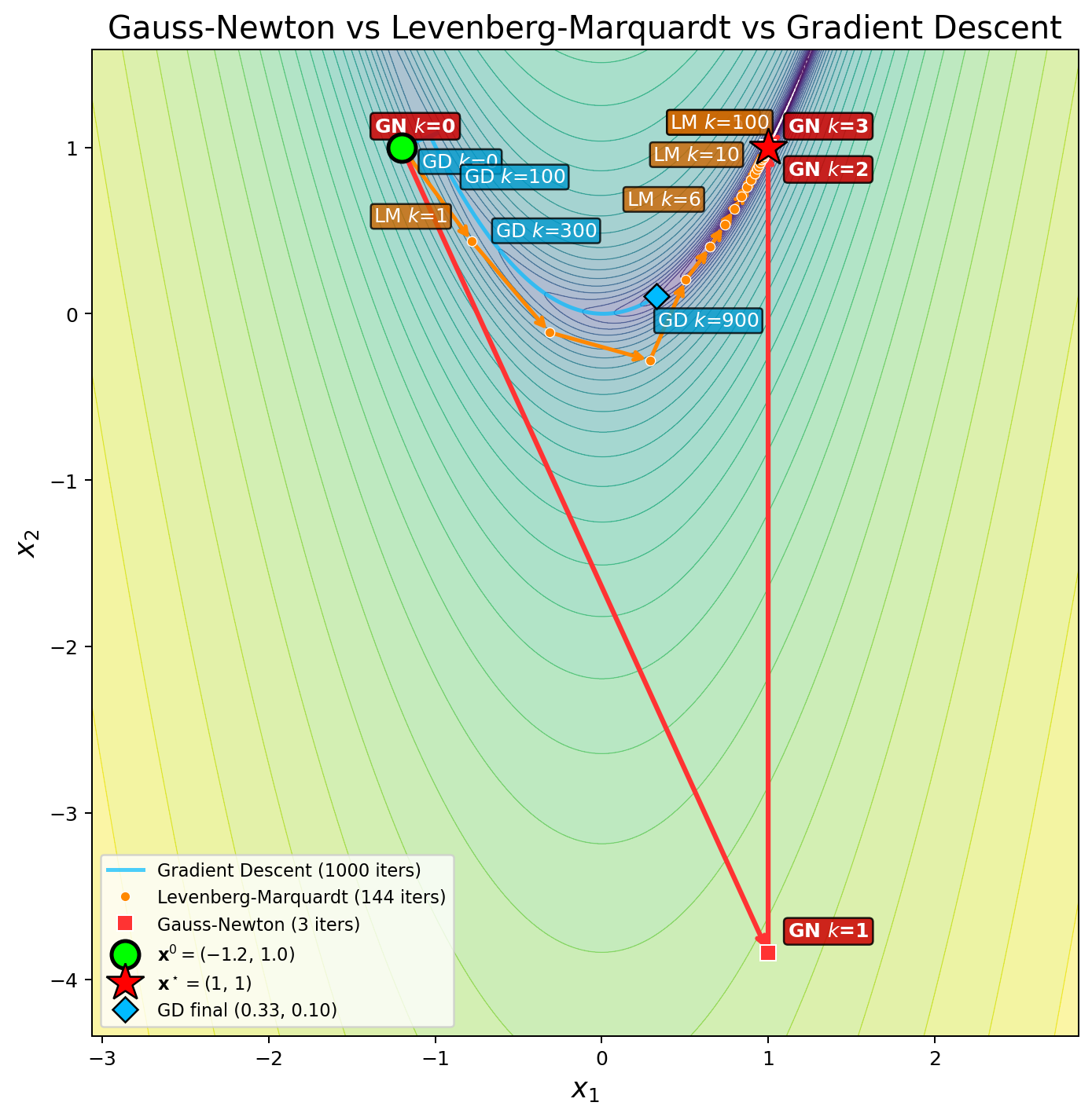
In common engineering problems, the optimization problem is to minimize the residual of a parametric model with respect to some observed data points.Given N...
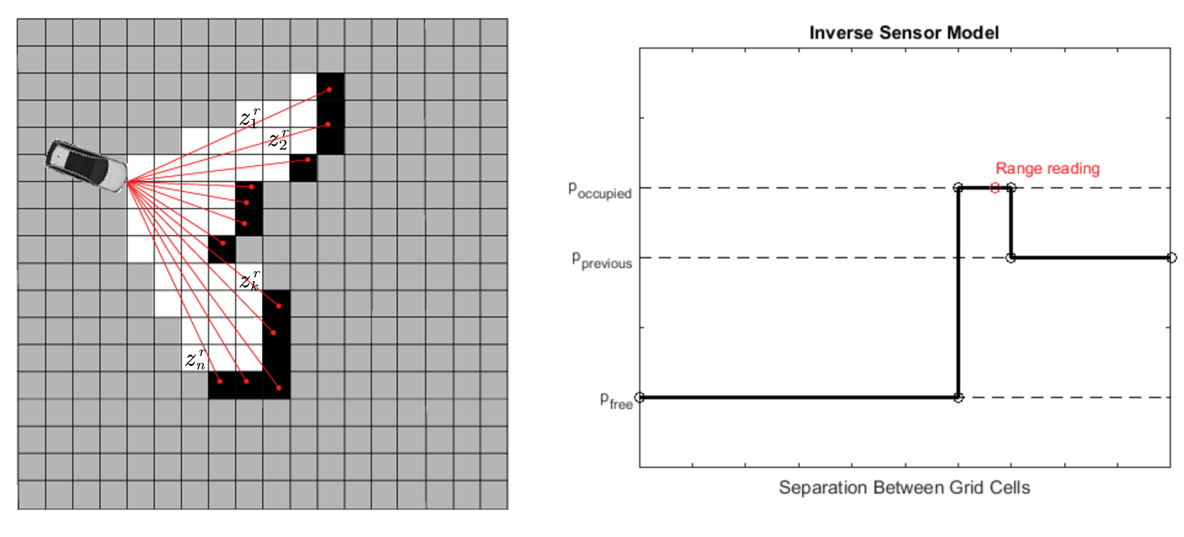
Besides state estimation or localization, which provide a robot with knowledge of where it is, it’s equally important for a mobile robot to perceive its surr...
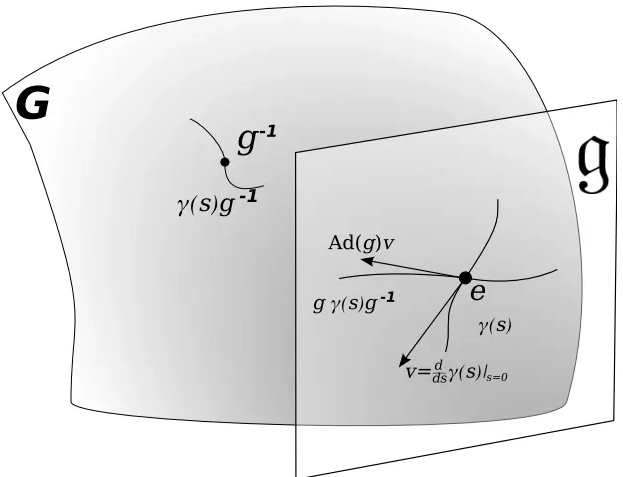
This note covers some of the fundamental concepts in Lie group and Lie algebra, and their applications to representing rigid body motion in robotics. A group...

In robot state estimation, the Bayes filter is a probabilistic approach that estimates the state from a sequence of controls and measurements by recursively ...