Solving ODEs by Series

7 minute read ·

Published: December 03, 2023

Now, we consider a somehow more general case, where we want to solve a linear second-order homogeneous equation with coefficients that are polynomials. Consider the following equation

p\left( t \right) y''+q\left( t \right) y'+r\left( t \right) y=0

where $p\left(t\right)\ne 0$ in some interval and $p\left(t\right),q\left(t\right),r\left(t\right)$ are polynomials of $t$ .

Properties of Power Series

An infinite series

y\left( t \right) =\sum_{n=0}^{\infty}{a_n\left( t-t_0 \right) ^n}=a_0+a_1x+a_2x^2+\cdots

is called a power series about $t=t_0$ . The following are some of its properties.

All power series have an interval of convergence. This means that there exists a nonnegative number $\rho$ such that the infinite series converges for $\left|t-t_0\right|<\rho$ , and diverges for $\left|t-t_0\right|>\rho$ . The number $\rho$ is called the radius of convergence of the power series.

The power series can be differentiated and integrated term by term, and the resultant series have the same radius of convergence.

One simple method to determine the radius of convergence of a power series is the Cauchy ratio test. Suppose

\underset{n\rightarrow \infty}{\lim}\left| \frac{a_{n+1}}{a_n} \right|=\lambda

Then the radius of convergence is $\displaystyle \rho=\frac{1}{\lambda}$ .

Many functions $f\left(t\right)$ that arise in applications can be expanded in power series, i.e., there exists a series of coefficients $a_0,a_1,a_2,\dots$ so that

f\left(t\right)=\sum_{n=0}^{\infty}a_n\left(t-t_0\right)^n

Such functions are said to be analytic at $t=t_0$ , the series expansion is called the Taylor series of $f$ about $t=t_0$ , and the coefficients can be found by

a_n=\frac{f^{\left(n\right)}\left(t_0\right)}{n!}

The radius of convergence can be determined if we treat the function $f$ in the complex plane. Let $z_0\in\mathbb{C}$ be the point that is closest to $t_0$ that $f^{(n)}(z_0)$ fails to exist, then the radius of convergence is $\rho=\left\|z_0-t_0\right\|$ .

The product of two power series is still a power series, this product is called the Cauchy product

\sum_{n=0}^{\infty}{a_n\left( t-t_0 \right) ^n}\sum_{n=0}^{\infty}{b_n\left( t-t_0 \right) ^n}=\sum_{n=0}^{\infty}{c_n\left( t-t_0 \right) ^n}

where the coefficient is

c_n=\sum_{j+k=n}a_jb_k=a_0b_n+a_1b_{n-1}+\cdots+a_nb_0

which is called the convolution of $a_n$ and $b_n$ .

Important series expansions (Remember them!)

\begin{align*} \frac{1}{1-x}=1+x+x^2+\cdots=\sum_{n=0}^{\infty}x^n, && \rho=1 \end{align*}

\begin{align*} e^x=1+x+\frac{x^2}{2}+\frac{x^3}{6}+\cdots=\sum_{n=0}^{\infty}\frac{x^n}{n!}, && \rho=\infty \end{align*}

\begin{align*} \sin x=x-\frac{x^3}{3!}+\frac{x^5}{5!}-\cdots=\sum_{n=0}^{\infty}\frac{\left(-1\right)^nx^{2n+1}}{\left(2n+1\right)!}, && \rho=\infty \end{align*}

\begin{align*} \cos x=1-\frac{x^2}{2!}+\frac{x^4}{4!}-\cdots=\sum_{n=0}^{\infty}\frac{\left(-1\right)^nx^{2n}}{\left(2n\right)!}, && \rho=\infty \end{align*}

\begin{align*} \ln\left(1-x\right)=-x-\frac{x^2}{2}-\frac{x^3}{3}-\cdots=-\sum_{n=1}^{\infty}\frac{x^n}{n}, && \rho = 1 \end{align*}

\begin{align*} \ln\left(1+x\right)=x-\frac{x^2}{2}+\frac{x^3}{3}-\cdots=\sum_{n=1}^{\infty}\left(-1\right)^{n+1}\frac{x^n}{n}, && \rho = 1 \end{align*}

Series Solution

For a second-order equation with variable coefficients (but are analytic functions, at least), although it’s not very rigorous, we can first expect that the solution $y$ is also a power series. Then, by doing series expansion and setting the polynomial coefficients properly, we can expect the equation to hold. A formal statement of this is as follows.

Let the functions $q\left(t\right)/p\left(t\right)$ and $r\left(t\right)/p\left(t\right)$ have convergent Taylor series expansions about $t=t_0$ , for $\left|t-t_0\right|<\rho$ . Then, every solution $y\left(t\right)$ of the differential equation

p\left(t\right)y''+q\left(t\right)y'+r\left(t\right)y=0

is analytic at $t=t_0$ , and the radius of convergence of its Taylor series expansion about $t=t_0$ is at least $\rho$ . Set

y\left(t\right)=a_0+a_1\left(t-t_0\right)+a_2\left(t-t_0\right)^2+\cdots

the coefficients are determined by plugging the expression into the differential equation and setting the sum of the coefficients of like powers of $t$ in this expression equal to zero.

Example (1)

However, it is possible that sometime $p\left(t_0\right)=0$ , and the above method of series expansion will fail to work, but we still want to find a solution around the point $t=t_0$ . One possible case is Euler’s equation.

Euler’s Equation

The differential equation

t^2y''+\alpha ty'+\beta y=0

where $\alpha,\beta\in\mathbb{R}$ are constant is known as Euler’s equation.

This equation has a singular point at $t=0$ and the series solution method above cannot work. However, we can treat $t>0$ and $t<0$ separately.

First, assume that $t>0$ .

For $t<0$ , let $t=-x$ ( $x>0$ ), and let $y=u\left(x\right)$ . Then the equation is transformed into

x^2u''+\alpha x u'+\beta u = 0

which should have the same solution as the case when $t>0$ . Thus, for the final solution, we only need to put a modulus on $t$ .

Observe that $t^2y''$ , $ty'$ , and $y$ will have the same order if $y=t^r$ . Our goal is to find two independent solutions. Therefore, we plug in $y=t^r$ into the equation.

\begin{align*} \frac{\mathrm{d}}{\mathrm{d}t}t^r=rt^{r-1}, && \frac{\mathrm{d}^2}{\mathrm{d}t^2}t^r=r\left(r-1\right)t^{r-2} \end{align*}

The original equation then becomes,

\left[r\left(r-1\right)+\alpha r+\beta\right]t^r=0

Hence, $y=t^r$ is a solution if and only if $r$ is a solution of the quadratic equation

r^2+\left(\alpha-1\right)r+\beta=0

Two Different Real Roots, $\left(\alpha-1\right)^2-4\beta >0$

The general solution is given by

y\left(t\right)=c_1t^{r_1}+c_2t^{r_t}

where $\displaystyle r_{1,2}=-\frac{1}{2}\left[\left(\alpha-1\right)\pm\sqrt{\left(\alpha - 1\right)^2-4\beta}\right]$ .

Two Equal Roots, $\left(\alpha-1\right)^2-4\beta =0$

One solution that is obvious is

y_1\left(t\right)=t^{r_1}

where $\displaystyle r=\frac{1-\alpha}{2}$ .

To find the second independent solution, applying the differential operator

\displaystyle L=t^2\frac{\mathrm{d}^2}{\mathrm{d}t^2}+\alpha t\frac{\mathrm{d}}{\mathrm{d}t}+\beta

and rewrite the equation as $Ly=0$ . Plug in $y=t^r$ , we have

L\left[t^{r}\right]=\left(r-r_1\right)^2t^{r}

Taking partial derivatives of both sides with respect to $r$ gives

\frac{\partial}{\partial r}L\left[t^r\right]=L\left[\frac{\partial}{\partial r}t^{r}\right]=\frac{\partial}{\partial r}\left[\left(r-r_1\right)^2t^r\right]

That is

L\left[t^r\ln t\right]=\left(r-r_1\right)^2t^r\ln t+2\left(r-r_1\right)t^r

We can see that if $r=r_1$ , then the right-hand side will vanish. Therefore, the second solution is

y_2\left(t\right)=t^{r_1}\ln t

The general solution is

y=\left(c_1+c_2\ln t\right)t^{r_1}

Two Complex Solutions, $\left(\alpha-1\right)^2-4\beta <0$

Let

\begin{align*} r_1=\lambda+i\mu, && r_2=\lambda-i\mu \end{align*}

and

\phi\left(t\right)=t^{\lambda+i\mu}=t^{\lambda}\left[\cos\left(\mu \ln t\right)+i\sin\left(\mu \ln t\right)\right]

It can be shown that the real and imaginary parts are two independent solutions. Therefore,

\begin{align*} y_1\left(t\right)=\mathrm{Re}\left(\phi\left(t\right)\right)=t^{\lambda}\cos\left(\mu\ln t\right)\\ y_2\left(t\right)=\mathrm{Im}\left(\phi\left(t\right)\right)=t^{\lambda}\sin\left(\mu\ln t\right)\\ \end{align*}

and the general solution is

y\left(t\right)=t^{\lambda}\left[c_1\cos\left(\mu\ln t\right)+c_2\sin\left(\mu\ln t\right)\right]

where $\displaystyle \lambda=\frac{1-\alpha}{2}$ , $\displaystyle \mu = \frac{\sqrt{4\beta-\left(\alpha-1\right)^2}}{2}$ .

Method of Frobenius

Here, we want to find a class of singular differential equations that is more general than Euler’s equation. A very natural generalization is the following

L(y)=y''+p\left(t\right)y'+q\left(t\right)y=0

where $p\left(t\right)$ and $q\left(t\right)$ can be expanded in series of the form

\begin{align*} p\left(t\right)&=\frac{p_{0}}{t}+p_1+p_2t+p_3t^2+\cdots\\ q\left(t\right)&=\frac{q_{0}}{t^2}+\frac{q_{1}}{t}+q_2+q_3t+q_4t^2+\cdots \end{align*}

In this case, the equation is said to have a regular singular point at $t=0$ . Equivalently, an equation has a regular singular point at $t=0$ if functions $tp\left(t\right)$ and $t^2q\left(t\right)$ are analytic at $t=0$ . It has a regular singular point at $t=t_0$ if functions $\left(t-t_0\right)p\left(t\right)$ and $\left(t-t_0\right)^2q\left(t\right)$ are analytic at $t=t_0$ .

We focus on the interval $t>0$ and multiply through the equation by $t^2$ and get

t^2y''+t\left(tp\left(t\right)\right)y'+t^2q\left(t\right)=0

Compare the above equation with Euler’s equation, and find that it seems like adding higher order terms, i.e., by changing $\alpha$ to $\displaystyle tp\left(t\right)=\sum_{n=0}^{\infty}p_nt^n$ , and changing $\beta$ to $\displaystyle t^2q\left(t\right)=\sum_{n=0}^{\infty}q_nt^n$ . Therefore, we may be able to obtain a solution by plugging in higher order term to the original $t^r$ solution. Specifically, let

y\left(t\right)=\sum_{n=0}^{\infty}a_nt^{n+r}=t^{r}\sum_{n=0}^{\infty}a_nt^n

Then,

y'\left(t\right)=\sum_{n=0}^{\infty}\left(n+r\right)a_nt^{n+r-1}

and

y''\left(t\right)=\sum_{n=0}^{\infty}\left(n+r\right)\left(n+r-1\right)a_nt^{n+r-2}

Plug these in the original equation at get

\begin{align*} L(y)&=t^r\left\{\sum_{t=0}^{\infty}\left(n+r\right)\left(n+r-1\right)a_nt^n+\left(\sum_{m=0}^{\infty}p_mt^m\right)\left[\sum_{n=0}^{\infty}\left(n+r\right)a_nt^n\right]\right\}\\ &+t^r\left(\sum_{m=0}^{\infty}q_mt^m\right)\left(\sum_{n=0}^{\infty}a_nt^{n}\right)\\ &=\left[r\left(r-1\right)+0_0r+q_0\right]a_0t^r\\ &+\left\{\left[\left(1+r\right)r+p_0\left(1+r\right)+q_0\right]a_1+\left(rp_1+q_1\right)a_0\right\}t^\\ &+\dots\\ &+\left(\left[\left(n+1\right)\left(n+r-1\right)+p_0\left(n+r\right)+q_0\right]a_n+\sum_{n=0}^{\infty}\left[(k+r)p_{n-k}+q_{n-k}\right]a_k\right)t^{n+r} \end{align*}

If we set

F\left(r\right)=r\left(r-1\right)+p_0r+q_0

and set the coefficient of each like power equal to zero, we have an indicial equation

F\left(r\right)=r\left(r-1\right)+p_0r+q_0=0

and a recurrence relation

F\left(n+r\right)a_n=-\sum_{k=0}^{n-1}\left[\left(k+r\right)p_{n-k}+q_{m-k}\right]a_k

From these two relations, we can (hopefully) obtain two sets of coefficients $a_n(r_1)$ and $a_n(r_2)$ and the two independent solutions are

\begin{align*} y_1\left(t\right)=t^{r_1}\sum_{n=0}^{\infty}a_n\left(r_1\right)t^{n}, && y_2\left(t\right)=t^{r_2}\sum_{n=0}^{\infty}a_n\left(r_2\right)t^{n} \end{align*}

if we can obtain two different real solutions $r_1$ and $r_2$ , with $\left(r_1-r_2\right)\notin\mathbb{Z}$ .

Next, we discuss the possible situations that the above conditions are not satisfied.

Two Complex Roots

If $r$ is a complex root of the indicial equation, then

y\left(t\right)=t^r\sum_{n=0}^{\infty}a_nt^{n}

is a complex-valued solution, whose real and imaginary part are both real-valued solutions.

Equal Roots

If $r$ is the only root of the indicial equation, then we have only one independent solution.

y_1\left(t\right)=t^r\sum_{n=0}^{\infty}a_nt^{n}

To find the other solution, use the similar method of dealing with Euler’s equation. The second solution is

y_2\left(t\right)=y_1\left(t\right)\ln t+\sum_{n=0}^{\infty}a_n'\left(r\right)t^{n+r}

Roots Differing by a Positive Integer

Suppose that $r_2$ and $r_1=r_2+N$ , where $N\in\mathbb{Z}^{+}$ , are two roots of the indicial equation. Then, we can certainly find one solution

y_1\left(t\right)=t^r\sum_{n=0}^{\infty}a_n\left(r_1\right)t^{n}

It may be impossible to find another solution with coefficients $a_n\left(r_2\right)$ .

In this case, the equation will have a second solution of the form

y_2\left(t\right)=ay_1\left(t\right)\ln t+\sum_{n=0}^{\infty}a_n'\left(r_2\right)t^{n+r_2}

Share on

Bluesky Facebook LinkedIn X (formerly Twitter)

You May Also Enjoy

Optimization Part 1 Basics and Least Squares

March 31, 2026 Mathematics

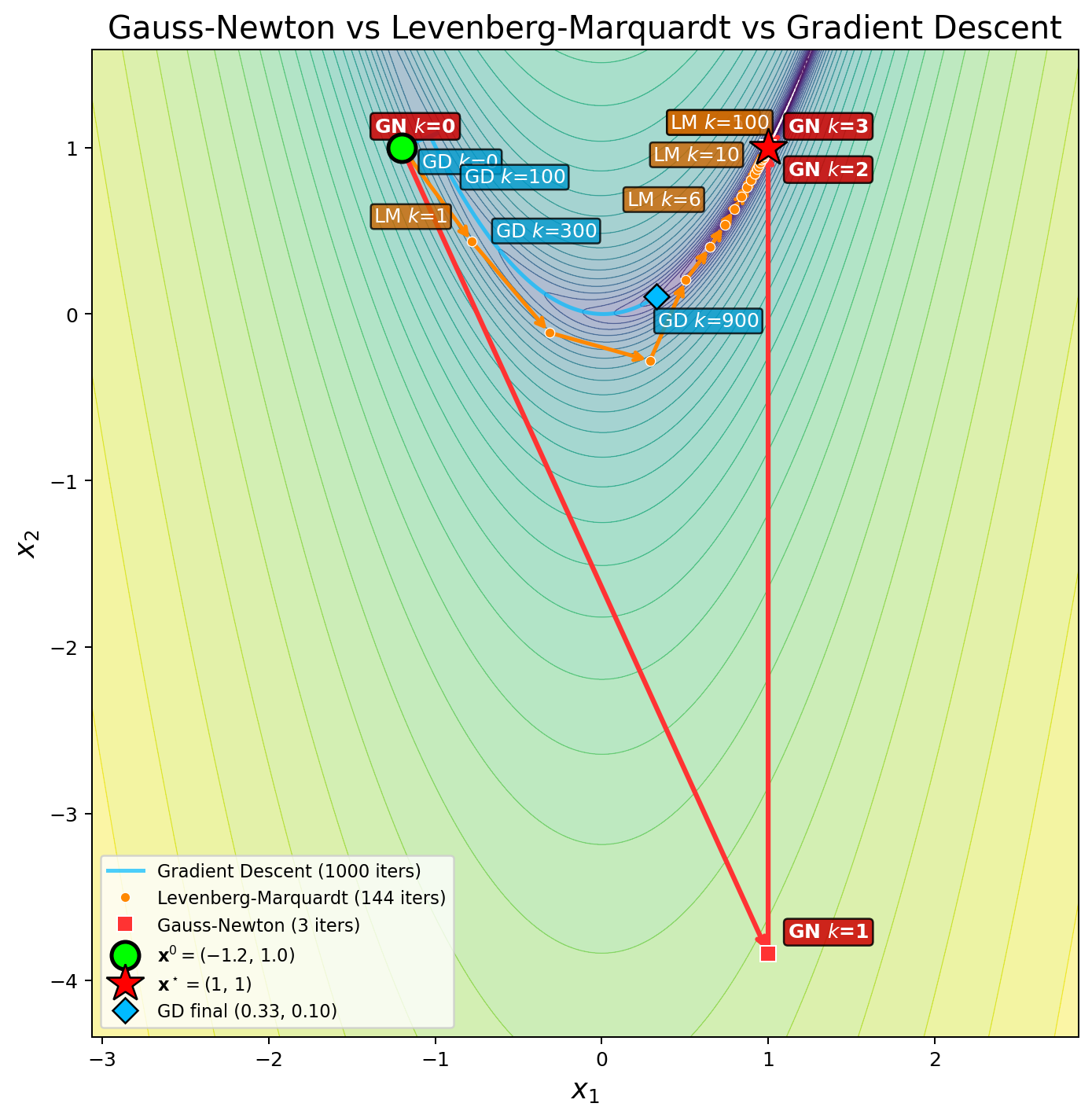
In common engineering problems, the optimization problem is to minimize the residual of a parametric model with respect to some observed data points.Given N...

Occupancy Grid Mapping

March 22, 2026 Robotics

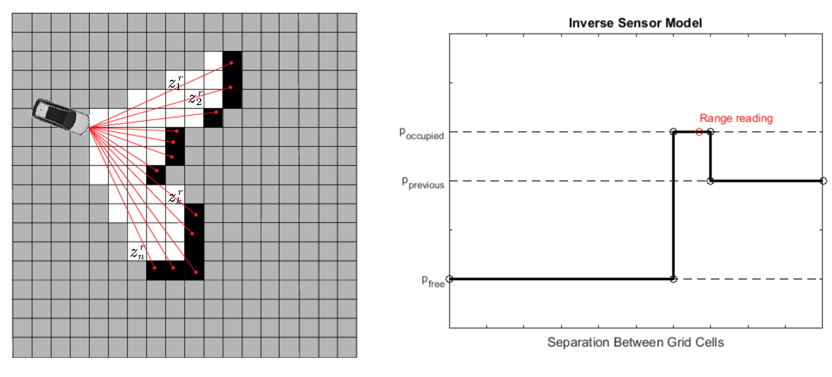
Besides state estimation or localization, which provide a robot with knowledge of where it is, it’s equally important for a mobile robot to perceive its surr...

Lie Theory in Robot Motion

March 10, 2026 Robotics

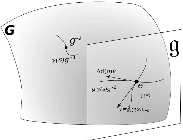
This note covers some of the fundamental concepts in Lie group and Lie algebra, and their applications to representing rigid body motion in robotics. A group...

Bayes Filtering and State Estimation

March 4, 2026 Robotics

In robot state estimation, the Bayes filter is a probabilistic approach that estimates the state from a sequence of controls and measurements by recursively ...

Guanyu Xu